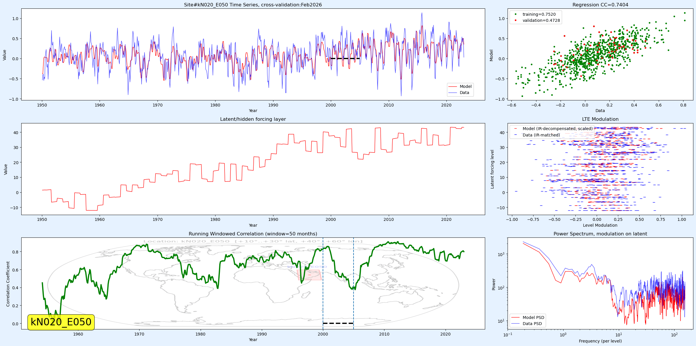
The chart below is a fit to a Kaplan SST quad using an LTE solution described in Chapter 12 of Mathematical Geoenergy¹. It may sound odd or counter-intuitive that the tides of an LTE formulation can impact temperature, but once you understand that most of the heat redistribution comes from mixing and upwelling of surface waters, then you realize the sources of forcing are limited — available from tides, winds, Coriolis effect, diurnal/seasonal cycles.

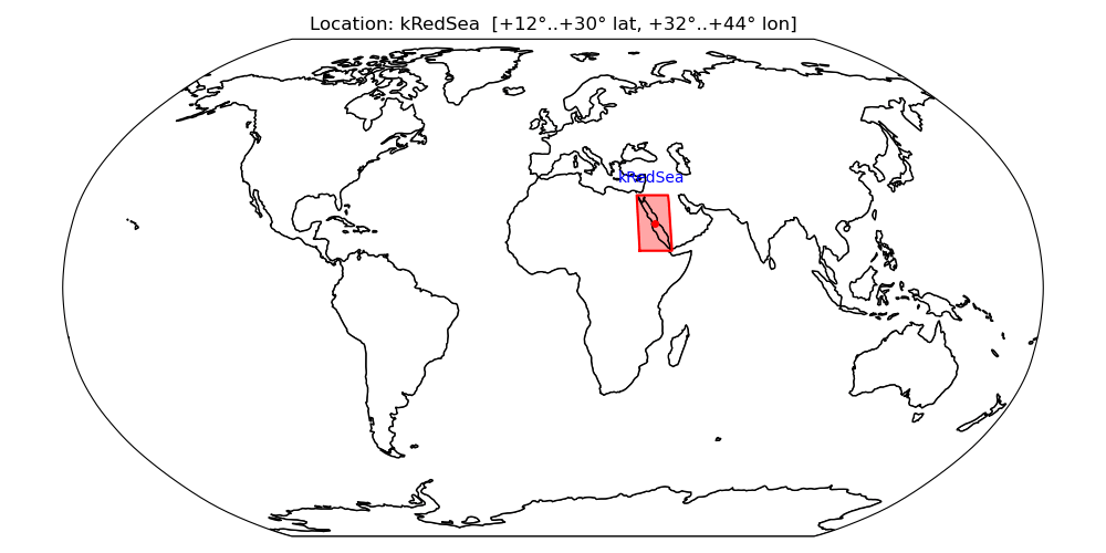
The region under study is the Kaplan SST quadrangle centered at 20°N, 50°E (10°N–30°N, 40°E–60°E), covering the Red Sea, the Gulf of Aden approach, the Persian Gulf, and the Gulf of Oman. Two narrow, sill-bounded straits gate exchange with the open ocean at either end of this box: Bab-el-Mandeb (Red Sea ↔ Gulf of Aden) and the Strait of Hormuz (Persian Gulf ↔ Gulf of Oman). This geometry — two shallow, evaporation-dominated seas each choked to the open ocean through a single narrow gap — is what makes the region interesting both to GEM-LTE‘s analysis and, independently, to a detailed basin hydrodynamics, which I won’t do but will cite later. Recall that the northernmost point of the Persian Gulf is one of the most unsurvivable parts of the world when it comes to heat index (and what is in store with global warming).

Red Sea / Persian Gulf Basin: a GEM-LTE case study

We look at this region in two passes — first a 1950–2023 fit, then the full 1856–2023 span.

1950+ model

From the PSL.NOAA.gov (N 20 E 50) we fit monthly Kaplan SST (877 points, 1950.0–2023.0) against GEM-LTE’s tidal forcing manifold with a held-out region 2000–2005 used only for post-hoc validation. The current production fit reaches r ≈ 0.74 data-vs-model correlation over the full 877-month span. That’s the chart at the top.

As stated, the region 2000–2005 was withheld from training, and the rolling-window correlation in the top chart dips specifically in the untrained gap and recovers immediately on both flanks (r ≈ 0.75 before, r ≈ 0.84 after) — the textbook signature of a genuine, non-leaking blocked holdout. It still looks good.

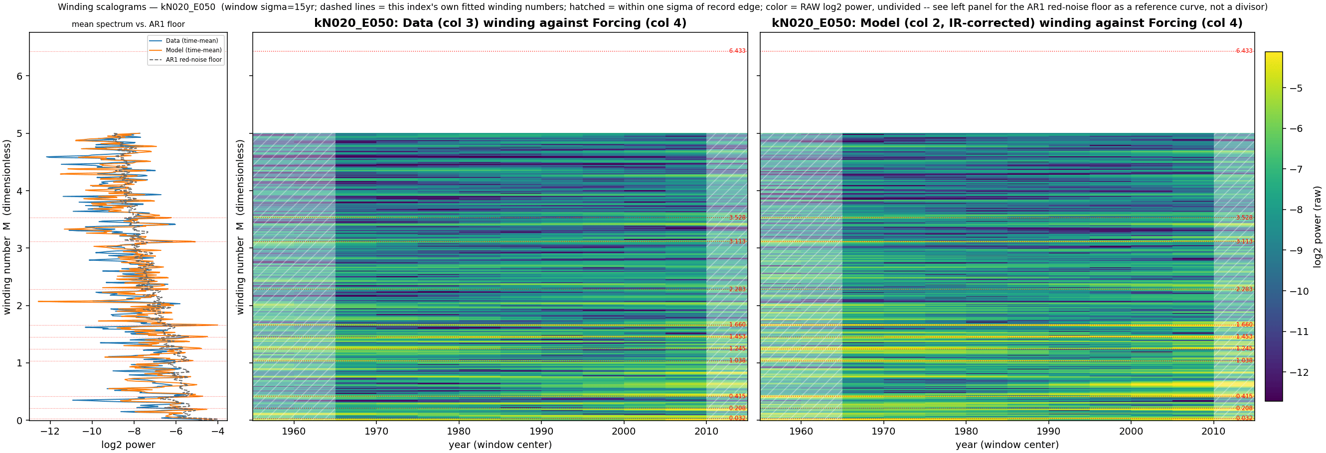
Winding structure

Every GEM-LTE index in this project shares one universal, spatially uniform global fundamental “backbone” term — and the Red Sea/Persian Gulf box is no exception: the same LOD calibrated forcing with a phase modulation term found independently in AMO, PDO, NAO, PNA, Baltic, etc. a common value (all 0.207–0.208). What distinguishes this region is the density of harmonics riding on top of that fundamental backbone — including [2, 5, 6, 7, 8, 11, 15, 17, 31], and several of the resulting winding rates (≈1.66, 1.87, 2.28, 2.90) show large, well-fit amplitudes with no analog in most other quads. Also have looked at the Gulf of Mexico and Aegean/Black Sea quad (as an aside there are distinguishable harmonic fingerprints between the Aegean and Black Sea just like there might for the Red Sea vs Persian Gulf, see more below).

Temporal power spectrum

A standard calendar-time periodogram (power_spectrum.py, AR(1) red-noise floor, 200 surrogates) gives a complementary view to the the forcing-domain winding scalogram above. The scalogram shows dense, persistent ridge structure across essentially the whole record; the plain frequency-domain view shows the model’s fidelity to the real data is spread out in several bands:

band (cyc/yr)	data’s share of its own variance	model/data power ratio
0.05–0.30 (multi-year)	0.225	0.52
0.30–0.70	0.146	0.37
0.70–1.30 (annual)	0.271	0.53
1.30–2.50	0.158	0.36
2.50–4.00	0.072	0.08
4.00–6.00 (sub-5-month)	0.041	0.06

According to the power spectrum below, the model isn’t capturing much of the signal faster than semi-annual.

Isolating just the model’s explicit seasonal regression terms (ann & sem — a fixed 1×/2× per-year sin/cos basis) and
comparing their own peak-to-peak excursion against the real data’s 1.0-to-(-1.0)-scale excursion confirms these terms together account for only roughly 10% of the real seasonal-cycle amplitude.

Having a subtle 10% annual cycle helps with the visual matching but the model capturing the erratic nature and having a strong cross-validation is the key finding.

The full 1856–2023 span

Kaplan SST’s ship-based (pre-satellite, pre-1950) coverage is patchy worldwide, but the Red Sea/Persian Gulf corridor is an exception: it has carried dense shipping traffic — and therefore dense ship-log SST sampling — since long before 1950, plausibly reinforced by Suez Canal traffic since 1869. That gives this region one of the longest trustworthy pre-satellite records in the whole 89-quad grid, and made it a natural candidate for a stationarity check that most other quads can’t support.

But to target the stationarity more precisely, I split that quad into a Persian Gulf area and a Red Sea area

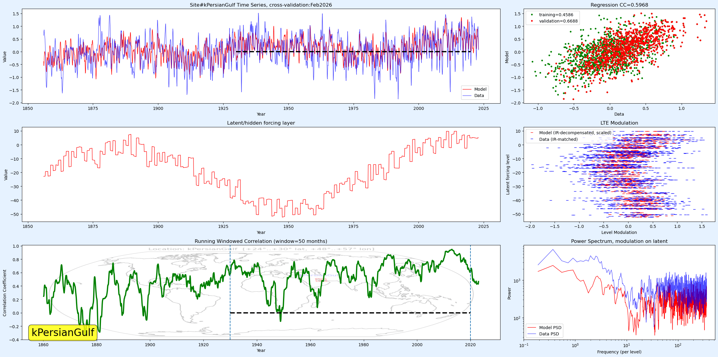
This the training on the Persian Gulf SST data with respect to the 1930-2020 manifold interval with automatic multiple linear regression on the winding sinusoids:

This is the lower range trained from 1860 to 1970:

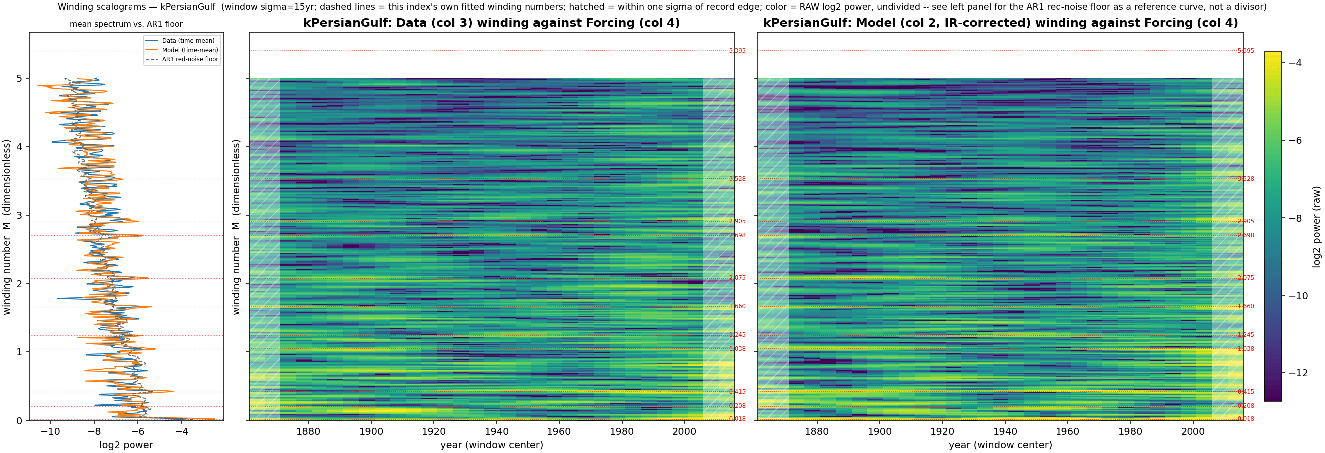
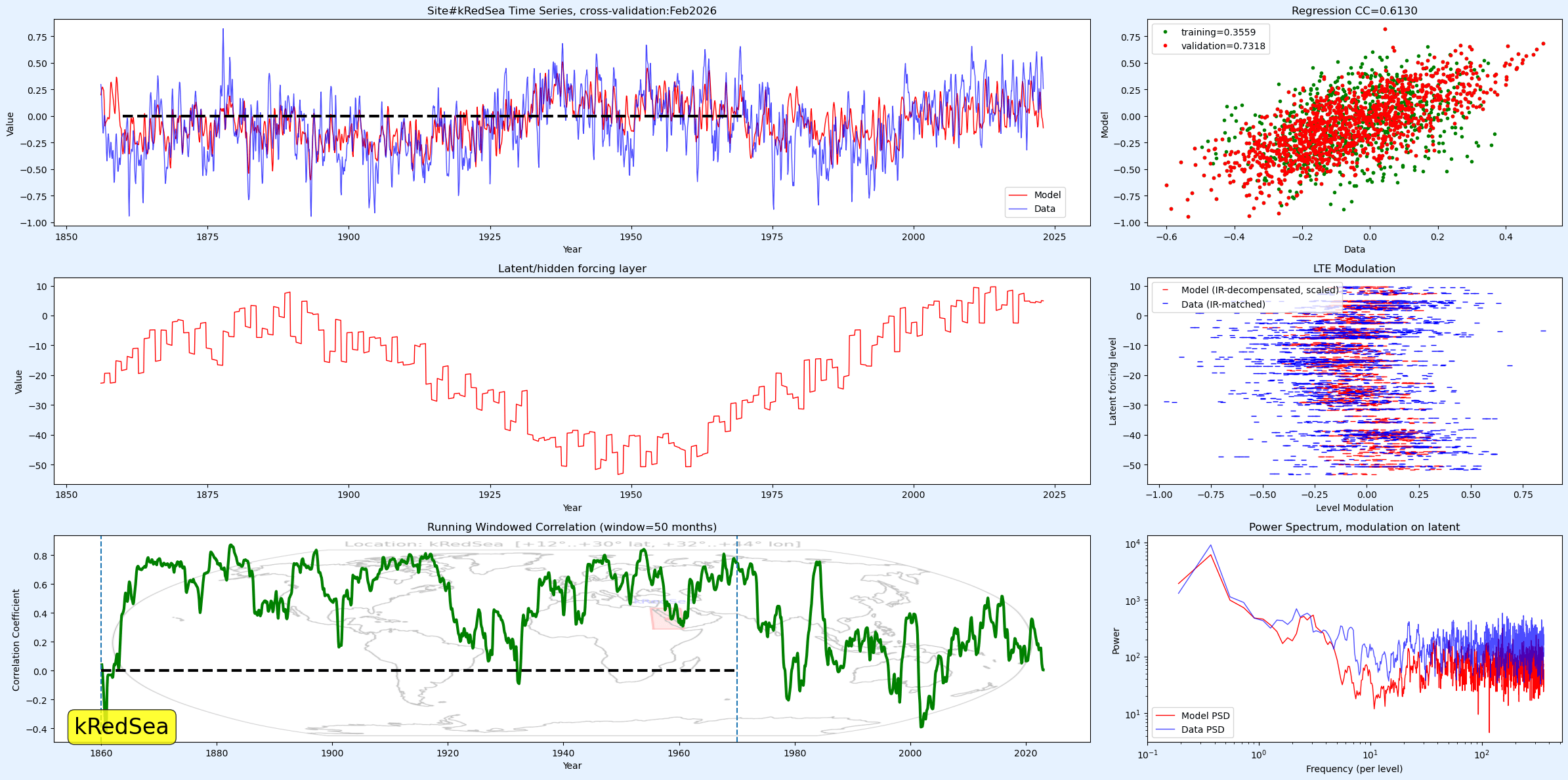
Two aspects to this (1) the ~60 year gradual modulation similar to AMO with the slow winding effectively doubling the frequency — the thought is that this is friction that rectifies the + and – excursions about the mean (2) the faster erratic cyclic excursions modeled by the higher winding harmonics. On both ends (with some overlap), the training reflects stationarity over the complementary validation interval. This is illustrated below showing the periodic harmonic comb that describes the windings (same as middle right panel above rotated by $90\degree$). Note that there are ~10 fundamental periods in 50 units so that the spacing is 4.77, but recall that the harmonic backbone is 0.2075 so that 4.77 * 0.2075 = 0.99 or the unitary $2\pi$ winding. The extra harmonics are part of the basin geometry that promote specific standing wave resonances. On the slower end, the longer winding modulation is what helps create the 120y to 60y frequency doubling. The bottom line is that this is a stationary periodic regime that when interacting with the specific tidal-driven forcing manifold leads to the seemingly erratic SST cycling. In fact, this is all likely highly deterministic, from the diurnal cycles to the annual cycles to these long-period LTE winding resonances, all paced by solar-seasonal and lunar-tidal cycles.

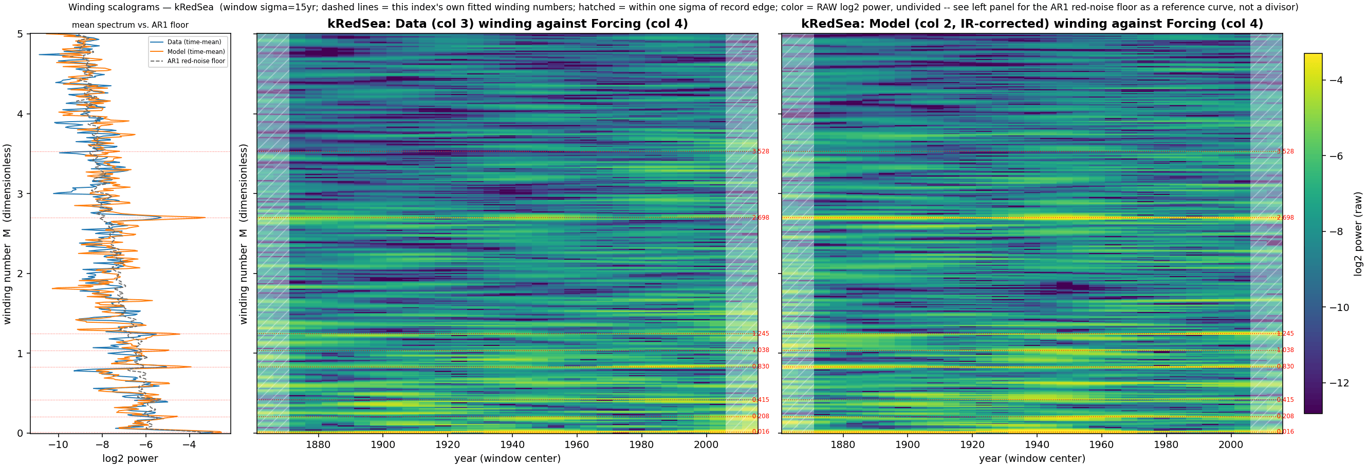
The continuity of the Persian Gulf winding scalogram structure is not quite as striking as for the Baltic MSL region. As shown below, long continuous ridges are not as apparent (except for the AMO-like low winding). Replacing that I think is more of a Moire pattern, representing the interference between multiple harmonic windings.

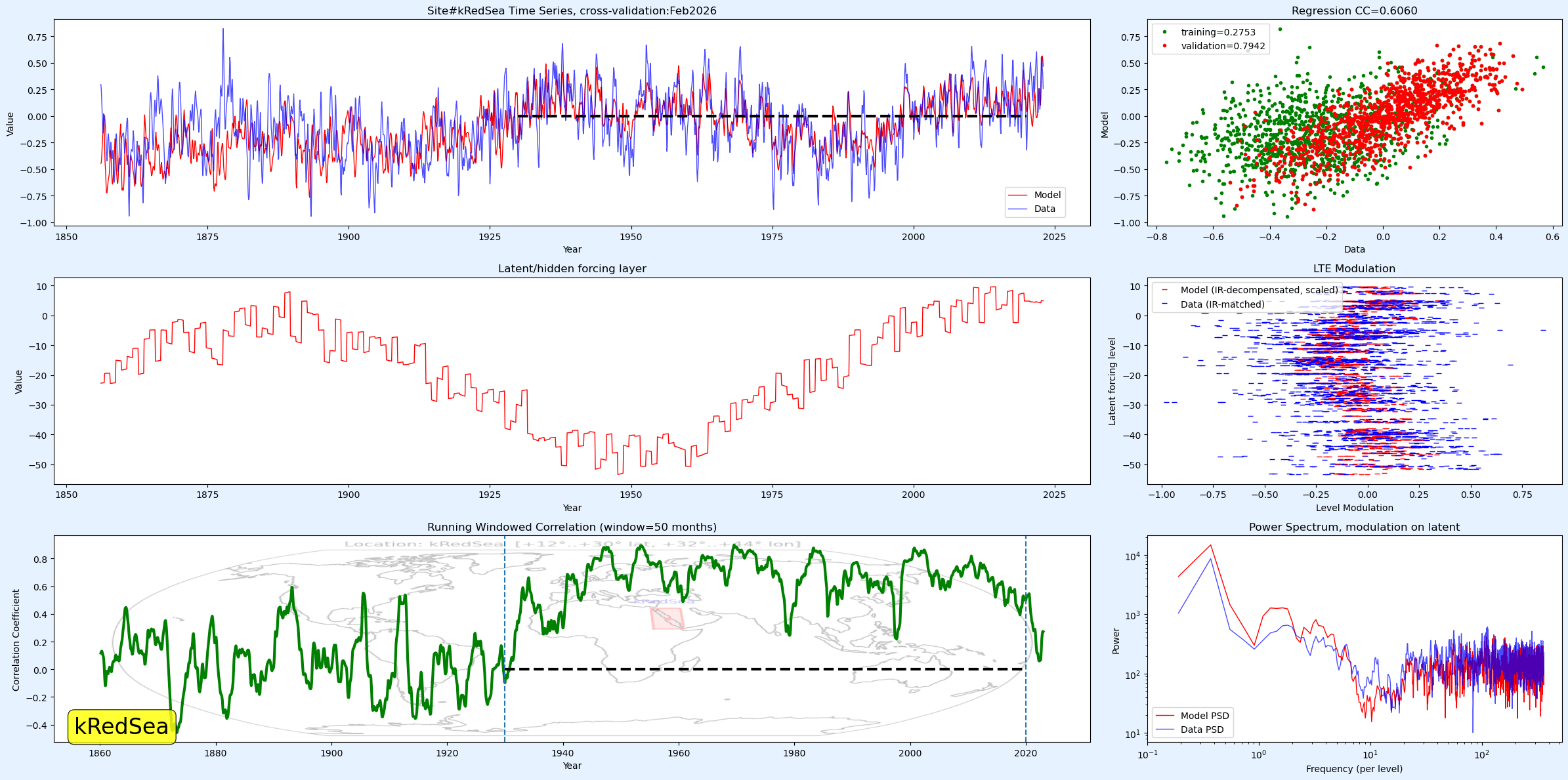
For the Red Sea, the effect is comparable, perhaps a little more prone to overfitting

Red Sea training 1930 to 2020

Red Sea training 1860:1970

The windings across the range remain stationary as the composition is more-or-less fixed as shown below. Again, it’s a mix of harmoncs

┌──────────────┬──────────────────┬─────────────┐
│ n (harmonic) │ Persian Gulf amp │ Red Sea amp │
├──────────────┼──────────────────┼─────────────┤
│  −0.08 (sub) │                  │      0.1125 │
├──────────────┼──────────────────┼─────────────┤
│   0.09 (sub) │           0.2912 │             │
├──────────────┼──────────────────┼─────────────┤
│   0.2075   1 │           0.0736 │      0.0677 │
├──────────────┼──────────────────┼─────────────┤
│            2 │           0.1812 │      0.0704 │
├──────────────┼──────────────────┼─────────────┤
│            4 │                  │      0.1180 │
├──────────────┼──────────────────┼─────────────┤
│            5 │           0.1101 │      0.0664 │
├──────────────┼──────────────────┼─────────────┤
│            6 │           0.1578 │      0.0253 │
├──────────────┼──────────────────┼─────────────┤
│            8 │           0.1788 │             │
├──────────────┼──────────────────┼─────────────┤
│           10 │           0.1071 │             │
├──────────────┼──────────────────┼─────────────┤
│           13 │           0.1475 │      0.1372 │
├──────────────┼──────────────────┼─────────────┤
│           14 │           0.0931 │             │
├──────────────┼──────────────────┼─────────────┤
│           17 │           0.0955 │      0.0341 │
├──────────────┼──────────────────┼─────────────┤
│           26 │           0.1065 │             │
└──────────────┴──────────────────┴─────────────┘

This is really an exercise of non-autonomously building a set of harmonics (and one subharmonic) that will transform the LOD calibrated forcing manifold into the observable SST. There are so many ways to get from A to B using non-linear formulations and whether this is the one that will always work remains to be seen.

The Aegean Sea/Black Sea pair

Before looking at Red Sea/Persian Gulf, this came up in the context of the Kaplan N040 E030 quad

Can split this data and found out that the Aegean portion is more dynamic.

Can see this when the windings composite is compared between the two. This barely touches the tip of the iceberg as all of these quads reveal interesting behavior.

---

Connecting to Lawen’s basin-dynamics work

I’ve been following Johannes Lawen’s fluid dynamics research on tidal dynamics within basins for some time. His numerical computations involve Voronoi-mesh-based, fully parallelized finite-volume coastal ocean code — shallow-water Navier–Stokes with Coriolis, viscous stress, and wave-resolving dynamics — built as an alternative to triangle-mesh models, and fast enough to exceed real-time performance on commodity hardware. Regarding this post on Tidal Basins, his recent published validation (2025, Ocean Science) is against tidal observations in Doha Bay, Qatar, inside the Persian Gulf half of this exact kN020_E050 quadrangle. Much of it is based on the faster diurnal scale including M2, S2, K1, and O1 tidal constituents which he configured to propagate through and dissipate within a narrow, strait-bounded shelf sea. That is precisely the class of problem the Red Sea and Persian Gulf pose: both are shallow seas gated to the open ocean through a single narrow sill (Bab-el-Mandeb, Hormuz). Lawen’s strait-dissipation framework gives a first-principles physical mechanism: a narrow sill acts as an impedance-mismatched gate that partially reflects incoming tidal energy, setting up a basin-scale standing structure with its own resonant frequencies, distinct from and generally higher-Q than open-shelf tidal response.

His research also involves surface heat exchange and evaporation. This is directly relevant here: the Red Sea and Persian Gulf are among the most strongly evaporative, negative-freshwater-budget semi-enclosed seas on Earth, each running a persistent two-layer exchange flow through its bounding strait (fresher, lighter inflow at the surface; saltier, denser outflow at depth) driven by basin-wide evaporative heat and salt loss. That overturning has its own natural annual rhythm, set by the seasonal cycle of evaporation and surface heating/cooling — a mechanistically impulsive, once-a-year-forced process, not a smooth sinusoidal insolation cycle. That is a plausible physical candidate for LTE modulation that I have long proposed: the finding that this region’s real seasonal SST shape is only ~10% explained by smooth annual/semi-annual harmonics, with the rest evidently riding on the tidal-modulated impulses, which then split off as satellite side-bands, losing the annual character .

How the two approaches relate. Perhaps GEM-LTE’s kN020_E050 fit and Lawen’s Wavedyne simulation are more different in kind, not degree. The GEM-LTE model here is a reduced-order, closed-form regression against a shared tidal-forcing manifold — a small number of winding rates and impulsive gates fit by direct linear/nonlinear regression, with no explicit representation of basin geometry, bathymetry, or momentum balance. Wavedyne is a resolved, first-principles finite volume solver of the actual momentum and continuity equations on a real mesh of the basin. I’ve tried running resolved shallow-water PDE side-studies alongside the empirical winding approach for AMO, QBO, PDO, NAO, PNA, and MSL— and the general pattern has been that the two lenses are complementary rather than competing: the resolved PDE can test whether a proposed physical mechanism is even dynamically plausible (e.g., whether Coriolis alone can produce a given resonance), while the winding regression is far cheaper to fit and can consume 150+ years of monthly data directly. At some point in the future, a Wavedyne-style resolved run of the Red Sea/Persian Gulf system with a realistic seasonal evaporation forcing, can be tuned against a regression model .

• Johannes Lawen — GHI, TU Hamburg-Harburg
• Wave-resolving Voronoi model of the Rouse number for sediment entrainment (Ocean Science, 2025)
• EGUsphere preprint of the above
• Yu, Yu, Wang, Kuang, Wang, Ding, Ito & Lawen (2017), “Tidal propagation and dissipation in the Taiwan Strait,” Continental Shelf Research 136:57-73
• environment.report (Lawen’s modeling portal)

Footnotes

1. Mathematical Geoenergy | Geophysical Monograph Series ↩︎