Ocean Dynamics History

The golden age in developing the theory for ocean dynamics spanned from 1775 to 1920. It was in 1775 that Pierre Simon-Laplace first developed simplified tidal equations. In historical terms this was considered the first “dynamic theory of tides” in which differential equations “describes the ocean’s real reaction to tidal forces“.   The golden age perhaps culminated with A.T. Doodson’s work in cataloguing 388 tidal frequencies — and which eventually formed the basis for establishing a consensus in understanding and predicting ocean tides.

In parallel to this work, pioneering research was carried out on the non-linear differential equations known as the Mathieu and Hills equations. The initial application of the Mathieu equation was for determining the harmonics of a vibrating drum head [1]. The Hills equation was more general and found application to perturbations to periodic orbits [2]. Lord Rayleigh independently investigated what was the Mathieu equation to understand the phenomena of period doubling [3]. Eventually, the Mathieu equation found its way to modeling the dynamics of ocean basins [4], but in retrospect that work appeared flawed and was much too specific in its scope given its peculiar Ansatz in trying to cast the ocean as an elliptical drumhead. Only later in 1954 did the fundamental application of the Mathieu equation to liquid sloshing become evident [5].

So it’s interesting to speculate how far one could have taken the prediction of ENSO dynamics by applying only this early knowledge and not paying attention to any new research beyond this point, circa ~1920. Hypothetically, we could have first applied Laplace’s tidal equations and solved it along the equator, giving this canonical form, where f(t) is a forcing:

ENSO = sin (k f(t))


Next, consider a canonical forced wave equation operating on the thermocline that has a Mathieu component and a 1-year delayed reinforcement, and a pair of stimuli corresponding to the Draconic (nodal) and Anomalistic (perigee/apogee) tidal forces.

f(t+Delta) = A cdot f(t) + M cdot cos(pi t + theta) cdot f(t) + K f(t- 1{year}) + F_{drac} (t) + F_{anom} (t)


The 1-year delay and the biennial modulation are an interesting combination in that they essentially work in conjunction to achieve a common collective effect. For example, if the constant M is reduced in scale, the constant K needs to be increased to achieve a similar result. This is essentially the same period doubling phenomena that Lord Rayleigh originally described. So, what the Mathieu modulation does is create an inducement for a biennial recurrence within the bulk fluid properties (gravity-induced, foreshadowing the modern sloshing models [6]), while the 1 year delay is a combined memory effect and positive-feedback perturbation to reinforce that biennial property (essentially a yearly high is followed by a yearly low, and vice versa).

So for values of A=0.785, M=0.3, K=-0.15 we can achieve a strong biennial modulation that also essentially recreates the ENSO behavior for the correct combination of seasonally-reinforced Draconic and Anomalistic signals. What’s more is that the seasonal-reinforcement adopts the inflection of the biennial modulation, acting as another positive feedback to maintain the long-term biennial model (see below).

Fig 1: Mathieu modulation and seasonal impulse. The seasonal impulse aligns with the sign (concave up or concave down) of the biennial modulation to enhance the lunar forcing driving the ENSO behavior.

The strong reinforcement always occurs in November/December of each year, but reverses in sign each year to follow the Mathieu modulation. This is an Ansatz, to be sure, but it effectively recreates the long-term behavior of ENSO, shown below.

Fig 2: If we assumed only knowledge of 1880 to 1920 and used that as a training region, the extrapolated fit reproduces the rest of the ENSO behavior remarkably well. And if a longer training interval is applied, the out-of-band fit improves. This is, as always, an issue with long-period basis functions.

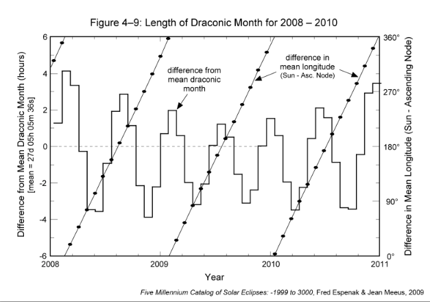
In the figure below we show the harmonic shape of the monthly lunar cycles. The fortnightly and 9-day harmonics are quite strong and when mixed as a multiplication, the bottom chart results. As I have asserted previously, the selectivity of the two periods is powerful. Applying anything other than precisely 27.2122 days for Draconic and 27.5545 days for Anomalistic and the fit rapidly degrades. Moreover, that also includes the phase shift of the cycles, which is necessary to align with the strongest nodal and apogee/perigee conditions.

That’s kind of a validation that someone with the brains of Laplace may have taken his original equations in this particular direction. Honestly, I’m not anywhere close to Laplace or Rayleigh in that department, but I do have access to a computer. That’s basically all it takes to reconstitute the old ideas in the new silicon age.

 
REFERENCES

[1] Mathieu, Émile. “Mémoire sur le mouvement vibratoire d’une membrane de forme elliptique.” Journal de mathématiques pures et appliquées 13 (1868): 137-203.

[2] Ince, Edward Lindsay. “On a general solution of Hills Equation.” Monthly Notices of the Royal Astronomical Society 75 (1915): 436-448.

[3] Rayleigh, Lord. “XXXIII. On maintained vibrations.” The London, Edinburgh, and Dublin Philosophical Magazine and Journal of Science 15.94 (1883): 229-235.

[4] S. Goldstein, “Tidal Motion in Rotating Elliptic Basins of Constant Depth.,” Geophysical Journal International, vol. 2, no. s4, pp. 213–232, 1929.

[5] Benjamin, T. Brooke, and F. Ursell. “The stability of the plane free surface of a liquid in vertical periodic motion.” Proceedings of the Royal Society of London A: Mathematical, Physical and Engineering Sciences. Vol. 225. No. 1163. The Royal Society, 1954.

[6] J. B. Frandsen, “Sloshing motions in excited tanks,” Journal of Computational Physics, vol. 196, no. 1, pp. 53–87, 2004.

The Lunar Geophysical Connection

The conjecture out of NASA JPL is that the moon has an impact on the climate greater than is currently understood:

Claire Perigaud (Caltech/JPL)
and
Has this research gone anywhere?  Looks as if has gone to this spin-off.
According to the current consensus, variability in wind is what contributes to forcing for behaviors such as the El Nino/Southern Oscillation (ENSO).
OK, but what forces the wind? No one can answer that apart from saying wind variability is just a part of the dynamic climate system.  And so we are lead to believe that a wind burst will cause an ENSO and then the ENSO event will create a significant disruptive transient to the climate much larger than the original wind stimulus. And that’s all due to positive feedback of some sort.
I am only paraphrasing the current consensus.
A much more plausible and parsimonious explanation lies with external lunar forcing reinforced by seasonal cycles.

Continue reading

ENSO and Noise

How do we determine confidence that we are not fitting to noise for the ENSO model ?  One way to do this is to compare the data against another model; in this case, a model that provides an instrumentally independent measure. One can judge data quality by comparing an index such as NINO34 against SOI, which are instrumentally independent measures (one based on temperature and one on atmospheric pressure).

If you look at a sliding correlation coefficient of these two indices along the complete interval, you will see certain years that are poorly correlated (see RED line below). Impressively, these are the same years that give poor agreement against the ENSO model (see BLUE line below). What this tells us is the poorly correlated years are ones with poor signal-to-noise ratio. But more importantly, it also indicates that the model is primarily fitting to the real ENSO signal (especially the peak values) and the noisy parts (closer to zero crossings or neutral ENSO conditions) are likely not contributing to the fit. And this is not a situation where the model will fit SOI better than NINO34 — because it doesn’t.

The tracking of SOI correlating to NINO34 matches that of Model to NINO34 across the range with the exception of some excursions during the 1950’s, where SOI fit NINO34 better that the model fit NINO34. The average correlation coefficient of SOI to NINO34 across the entire range is 0.75 while the model against NINO34 is less but depending on the parameterization always above 0.6.

As a result of this finding, I started to use a modification of a correlation coefficient called a weighted correlation coefficient, whereby the third parameter set is a density function that remains near 1 when the signal-to-noise (SNR) ratio is high and closer to zero where the SNR is closer to zero. This allows the fit to concentrate on the intervals of strong SNR, thus reducing the possibility of over-fitting against noise.


Or is it really all noise?   (Added: 5/17/2017)

As I derived earlier, the solution to Laplace’s tidal equations at the equator for a behavior such as QBO leads to a sin(k sin(f(t))) modulated time-series, where the inner sinusoid is essentially the forcing. This particular formulation (referred to as the sin-sin envelope) has interesting properties. For one, it has an amplitude limiting property due to the fact that a sinuosoid can’t exceed an amplitude of unity. Besides this excursion-limiting behavior, this formulation can also show amplitude folding at the positive and negative extremes. In other words, if the amplitude is too large, the outer sin modulation starts to shrink the excursion, instead of just limiting it. So if there is a massive amplitude, what happens is that the folding will occur multiple times within the peak interval, thus resulting in a rapid up and down oscillation. This potentially can have the appearance of noise as the oscillations are so rapid that (1) they may blur the data record or (2) may be unsustainable and lead to some form of wave-breaking.  I am not sure if the latter is related to folding of geological strata.

So the question is: can this happen for ENSO? I have been feeding the solution to the delayed differential Mathieu equation as a forcing to the sin-sin envelope and find that it works effectively to match the “noisy” regions identified above.  In the figure below, the diamonds represent intervals with the poorest correlation between NINO34 and SOI and perhaps the noisiest in terms of SOI. In particular, the regions labelled 1 and 6 indicate rapid cyclic excursions.

By comparison, the model fit to ENSO shows the rapid oscillations near many of the same regions. In particular look at intervals indicated by diamonds 1 and 6 below, as well as the interval just before 1950.

Now, consider that these just happen to be the same regions that the ENSO model shows excessive amplitude folding.  The pattern isn’t 100% but also doesn’t appear to be coincidental, nor is it biased or forced (as the fitting procedure has no idea that these are considered the noisy intervals).  So the suggestion is that these are points in time that could have developed into massive El Nino or La Nina, but didn’t because the forcing amplitude became folded. Thus they could not grow and instead the strong lunar gravitational forcing went into rapid oscillations which dissipated that energy. In fact, it’s really the rate of change in the kinetic energy that scales with forcing, and the rapid oscillations identify that change. Connecting back to the theory, that’s what the sin-sin envelope describes — its essentially a solution to a Hamiltonian that conserves the energy of the system. From the Sturm-Liouville equation that Laplace’s tidal equations reduce to, this answer is analytically precise and provided in closed-form.

The caveat to this idea of course is that no one else in climate science is even close to considering such a sin-sin formulation.  Consider this:

… yet …

An alternative model that matches ENSO does not exist, so there is nothing at the moment to refute.  And see above how it fits in balance with known physics.

ENSO Proxy Validation

This is a straightforward validation of the ENSO model presented at last December’s AGU.

What I did was use the modern instrumental record of ENSO — the NINO34 data set — as a training interval, and then tested across the historical coral proxy record — the UEP data set.

The correlation coefficient in the out-of-band region of 1650 to 1880 is excellent, considering that only two RHS lunar periods (draconic and anomalistic month) are used for forcing. As a matter of fact, trying to get any kind of agreement with the UEP using an arbitrary set of sine waves is problematic as the time-series appears nearly chaotic and thus requires may Fourier components to fit. With the ENSO model in place, the alignment with the data is automatic. It predicts the strong El Nino in 1877-1878 and then nearly everything before that.

Continue reading

ENSO and Tidal SLH – A Biennial Connection

[mathjax]It’s becoming abundantly clear that ENSO is driven by lunisolar mechanisms, especially true considering that we use the preferred models describing sloshing of water volumes — the Mathieu equation and the delay differential equation. What’s more, given the fact that the ENSO model works so well, one can guess that a connection between ENSO and lunar tidal forces should carry over to models for historical sea-level height (SLH) tidal data.

From my preliminary work analyzing SLH tidal data in 2014, I found an intriguing pattern relating to the same biennial pattern observed in the ENSO model. An extract from that post is reproduced below:

“The idea, related to delay differential equations, is to determine if it is at all possible to model at least part of ENSO (through the SOI) with data from a point in time in the tidal record with a compensated point from the past. This essentially models the effect of the current wave being cancelled partially by the reflection of a previous wave.

This is essentially suggesting that $$SOI = k f(t) – k f(t-Delta t)$$ where f(t) is the tidal record and k is a constant.

After some experimenting, a good fit is obtained when the current tidal data is set to 3 months ago, and the prior data is taken from 26 months in the past. To model the negative of ENSO, the 3-month old data is subtracted from the 26-month old data, Figure 1:”

Fig 1: Model of ENSO uses Tidal Gauge readings from Sydney Harbor.

This observation suggests a biennial pattern whereby high correlations in the time series occur for events observed close to two-years apart, with the difference taken up by the ENSO signal. The latter is at least partly due to the inverted barometer effect on SLH.

The sensitivity of the biennial effect is shown in the following contour diagram, where the peak CC is indicated and a slanted line showing the 2-year differencing points (table of the correlation coefficients here)

Focussing on the mechanisms for the correlation, the predictor can be reformulated as

f(t) = f(t-Delta t) + SOI / k


or that the 2-year prior SLH reading, with the addition of the SOI signal, will accurately represent the current SLH reading subject to a ~3 month lag.

My thinking is that this correlation can only occur if there is an actual biennial signal in the SLH itself. We can mathematically conjecture what is happening with the two year differencing by assuming that the SLH has the same height offset whenever pairs of points are separated by two years. You can see this in the following figure:

This brings up an interesting question as to why this biennial signal apparently can’t be detected via conventional means. A likely guess is because it gets obscured by the ENSO signal. And since the ENSO signal has never been adequately modeled, no one has an inkling that a biennial signal coexists in the mix. Yet this unconventional delay differencing approach (incidentally discovered with the help of machine learning) is able to discern it with a strong statistical significance.

The gist of this discovery is that a biennial tidal SLH motion exists and likely contributes (or at least identifies) the nonlinear biennial modulation driving the ENSO model described in previous posts.

Summary:

ENSO has elements of an annual teeter-totter. If you look through the research literature, you will find numerous references to a hypothesized behavior that one annual peak is followed by a lesser peak the next year. Yet, no evidence that this strict biennial cycle is evidence in the data — it’s more of a hand-wavy physical argument that this can or should occur.

The way to model this teeter-totter behavior is via Mathieu equations and delay differential equations. Both of these provide a kind of non-linear modulation that can sustain a biennial feedback mechanism.

The other ingredient is a forcing mechanism. The current literature appears to agree that this is due to prevailing wind bursts, which to me seems intuitive but doesn’t answer what forces the wind in the first place. As it turns out, only two parameters are needed to force the DiffEq and these align precisely with the primary lunar cycles that govern transverse and longitudinal directional momentum, the draconic and anomalistic months.

The ENSO model turns into a metrology tool

Note the following table and how the draconic and anomalistic values zone in on the true value when correlating model against data:

Fitting the DiffEq values progressively away from the true value for the lunar tidal cycle results in a smaller correlation coefficient.

Having one of these values align may be coincidence, but having both combine with that kind of resolution is telling. The biennial connection to SLH tidal measurements is substantiation that a biennial modulation is intrinsic to the physical process.

The ENSO model turns into a metrology tool

When the model is able to discern values of fundamental physical constants to high precision, it has ceased to become of hypothetical interest and transformed into one of practical significance and of essentially able to determine ground truth.

The ENSO model is a Mathieu differential equation with a biennial modulation and an added delay differential of one year. The DiffEq is this :

f''(t) +gamma f'(t) + omega_o^2 cdot ( alpha + beta cos( pi t +theta)) cdot f(t) + K cdot f(t-1{year}) = F(t)


This is solved with a straightforward differential expansion

f(t+Delta) = A cdot f(t) + B cdot f(t- Delta t) + C cdot f(t- 2 Delta t) + M cdot cos(pi t + theta) cdot f(t) + K f(t- 1{year}) + F_{drac} (t) + F_{anom} (t)


The resultant f(t) is compared to the NINO34 time series by maximizing the correlation coefficient. All the DiffEq parameters are allowed to vary (constrained to the appropriate sign for feedback parameters) and also the two unknown forcing periods corresponding to what we hypothesize as the strongly seasonally-pulsed Draconic and Anomalistic cycles (the Tropical/Synodic/Sidereal cycle is not considered first-order as a global effect). With minimal filtering of the NINO34 signal over the range of 1880 to present day, the correlation coefficient reaches upwards of 0.65 with a clearly obvious peak matching.

The DiffEq iterative solver is only constrained such that the Draconic and Anomalistic periods are close to the known cycles of 27.21222082 and 27.55454988 days. So we constrain them to the following intervals and find out whether the solver homes in on the actual values.

27.2 leq {Drac} leq 27.3

27.5 leq {Anom} leq 27.6


This is respect to an average calendar year of 365.2422 days. (As an aside, this computation is so sensitive that knowledge of leap years has a real impact)

We also clamp the unknown phases to a known value of the node crossing (for Draconic) and of a known value of a perigee point (for Anomalistic). This does not influence the precise knowledge of the unknown cycle period but supplying this particular ansatz prevents the solver from wandering around too much and giving a strong hint as to where to phase align the two cycles.

Incredibly, the results after about an hour’s worth of computation gives

Drac = 27.21178772 days

Anom = 27.55490106 days

This precision amount to predicting the Draconic lunar month period to within 37 seconds and the Anomalistic lunar month to within 30 seconds. This is with respect to a starting search window of 0.1 day or 2.4 hours, which is 8640 seconds, thus winnowing down the initial guess to a much finer resolution. So, if this was a random chance occurrence it would have a probability of (37/8640)*(30/8640) = 0.000015 to occur within that error margin. Remember that both periods match closely and are independent so the likelihoods are multiplied. That gives a 1 in over 60,000 chance of a random draw falling within that margin. Moreover, this value gives a strong peak in the correlation coefficient, falling off quickly away from these values. For a 30 second accumulated error per lunar month, this when propagated over ~1800 lunar months in a ~130 year interval will lead to a 15 hour error, or 15/24 out of 27 days, which is about a 0.15 radian propagated error. For comparison, 1.57 radians is needed to cause the phase to interfere destructively against the true value of the detected lunar month over this long interval. But cosine(0.15) is 0.99, which will give only a weak 1% of the worst case destructive interference.

As it stands the result is deterministically repeatable, as it will hone in on the same periods independent of a seed value. Evidently, the 1800 lunar months in the ENSO series is enough to provide a high resolution determination of its value — this is the equivalent to taking sea-level height tidal readings over many months to extract the diurnal or semi-diurnal periods. The difference is that this ENSO analysis is detecting the monthly long-period tidal values and not the much more convenient daily tidal data.

The significance of the described model and the associated results should not be undersold. The ENSO time series record obviously tracks the primary lunar cycles to such an extent that the model becomes an extremely sensitive metrology tool for indirectly estimating the lunar periods. (The direct measurement is obviously done though visual or sensor-based lunar tracking techniques, the most rudimentary of which has been known for centuries)

And bottom-line, realistically anybody can do this computation — as supplemental guide, a spreadsheet was supplied in the previous post . It’s all data driven and there really is no hands-on manipulation except a nudge to point the computation in the right direction. Odds are in favor that everyone that tries will find the same result, much like a tidal analysis will generate an identical result for the primary constituent periodic factors.

Unfortunately, the perceptions of a tidal period contributing to a clearly regular and discernible pattern (see this) remains a powerful incentive to question the results.  Yet, no one is under the pretense that a non-linear model will produce an obviously periodic pattern either. It’s really a case of a cyclic attractor that is stationary and stable,  and thus conducive to predictive modeling. Contrary to what the climate science deniers such as Judith Curry and Anastasios Tsonis assert, ENSO may not really be that complicated.