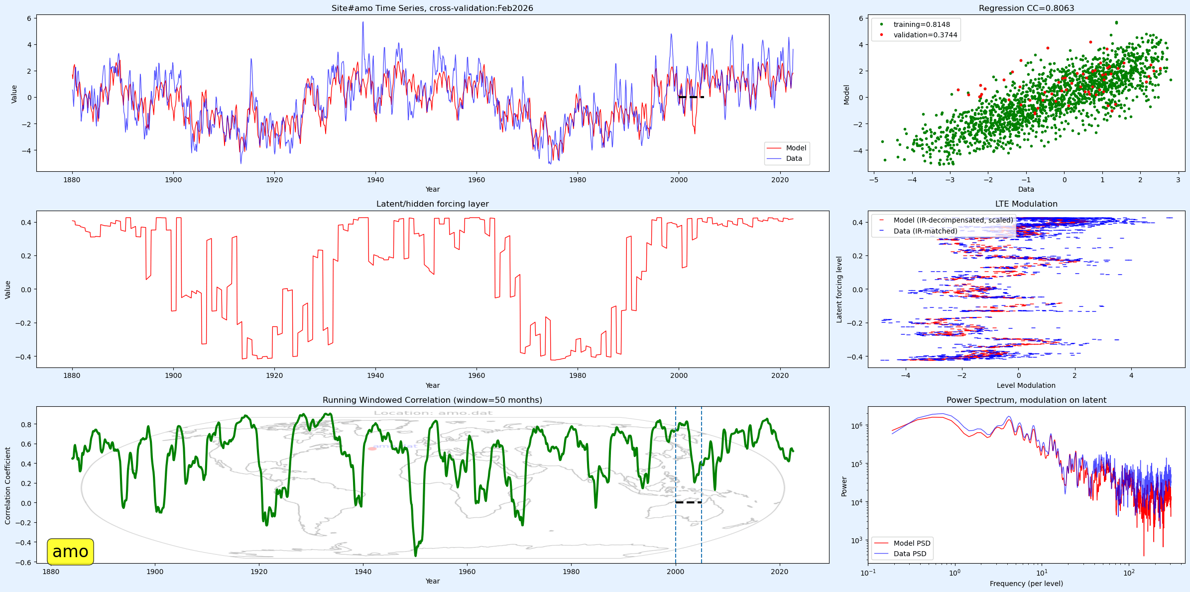
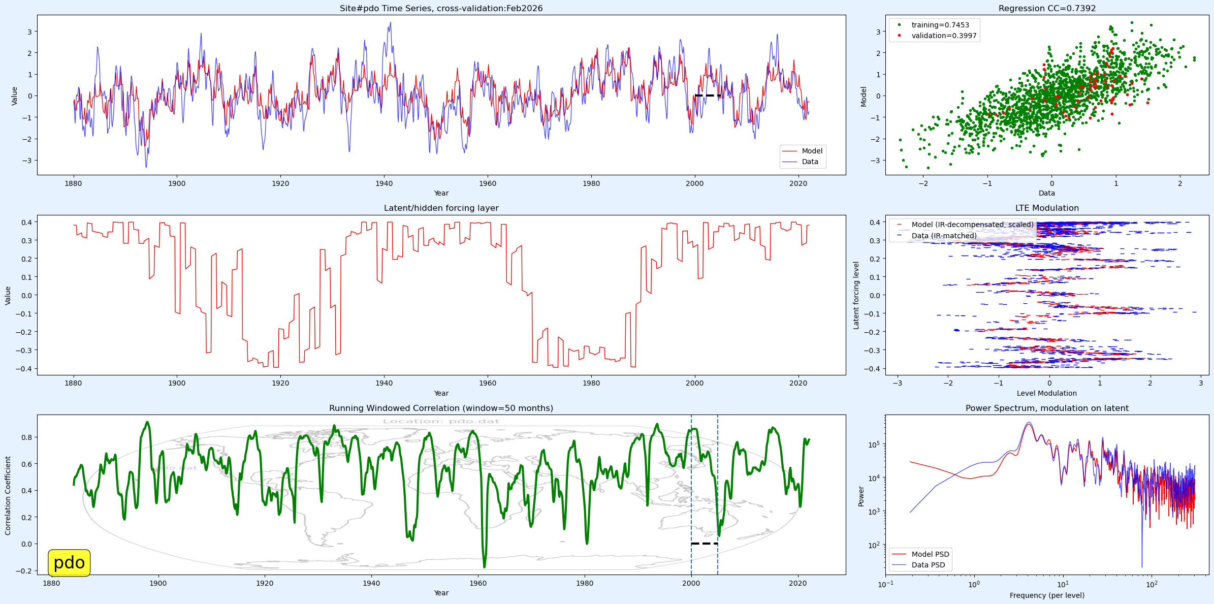
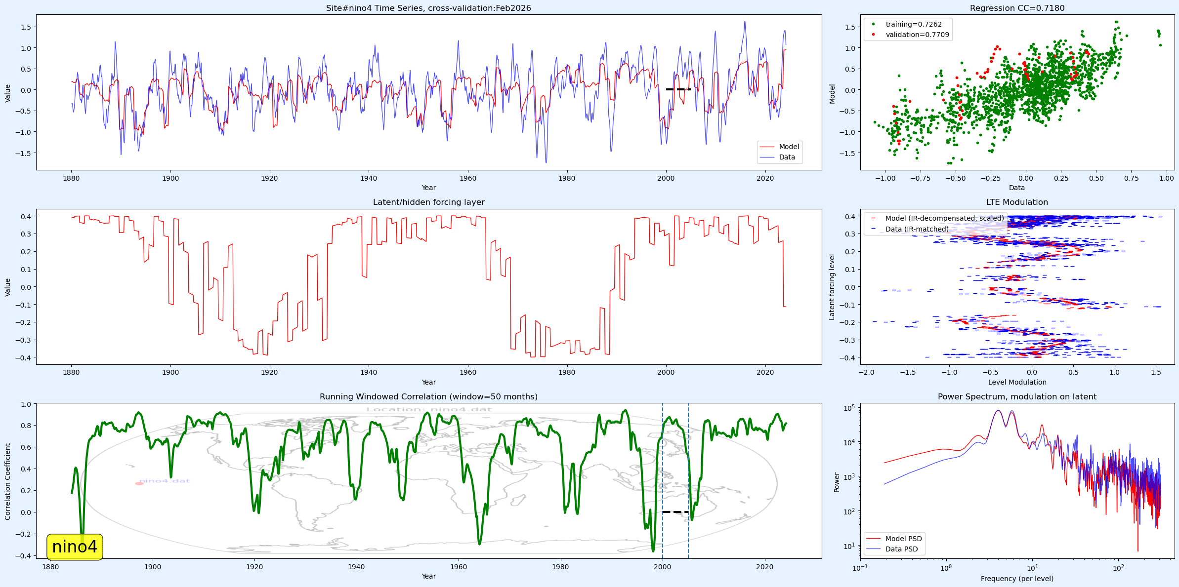
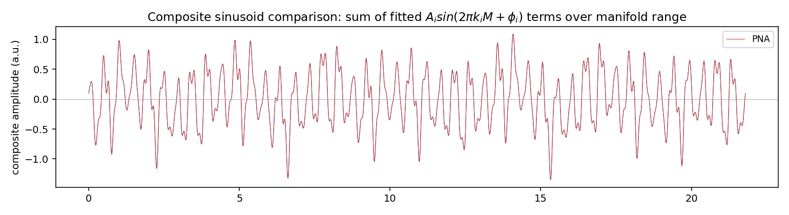
With the correct intermediate manifold, those of AMO and PDO are nearly indistinguishable. The ocean response is subtle — AMO has the basin-wide slow response, whereas PDO doesn’t, and both have a similar LTE modulation as shown in the middle-right panel below.
This is not a teleconnection but a common-mode forcing manifold each with a distinct response.
All the quads in the global SST grid follow from these two as seeded values and with NINO4, which seems to have more of a split winding character than PDO – see experiments/Oct2026_layer_ir
The essential fitting equation is the following, where is the integrated annual impulse response to the calibrated LOD tidal forcing1. The term is a spherical fitted sinusoidal phase correction. The winding is small and represents the basin friction layer. For AMO, the sum is essentially a single winding and with ENSO, a second winding emerges so .
Model =
where
This cascaded sinusoidal modulation is not complex norcomputational-intensive in comparison to a GCM
Probably doesn't but a full CFD climate simulation (GCM) using the fastest supercomputer takes the power of keeping a 737 flying at altitude. That's an exaflop of computing.
And an empirical neural network representation, which features an analogous set of convolutional layers, would be impossible to reverse engineer.
Global SST
The variations observed in global SST are largely accounted for by the ENSO, AMO, and PDO indices. A linear trend, corresponding to AGW, is needed to model global SST below, of which the model is a composite of all the modeled quads in the Kaplan extend SST V2.
“ As a pattern of internal climate variability, the state of the PNA occasionally changes without a clear and identifiable cause. This reduces the predictability of the PNA and can complicate long-range seasonal weather forecasts. Predictability of the PNA is limited to roughly within 10 days“
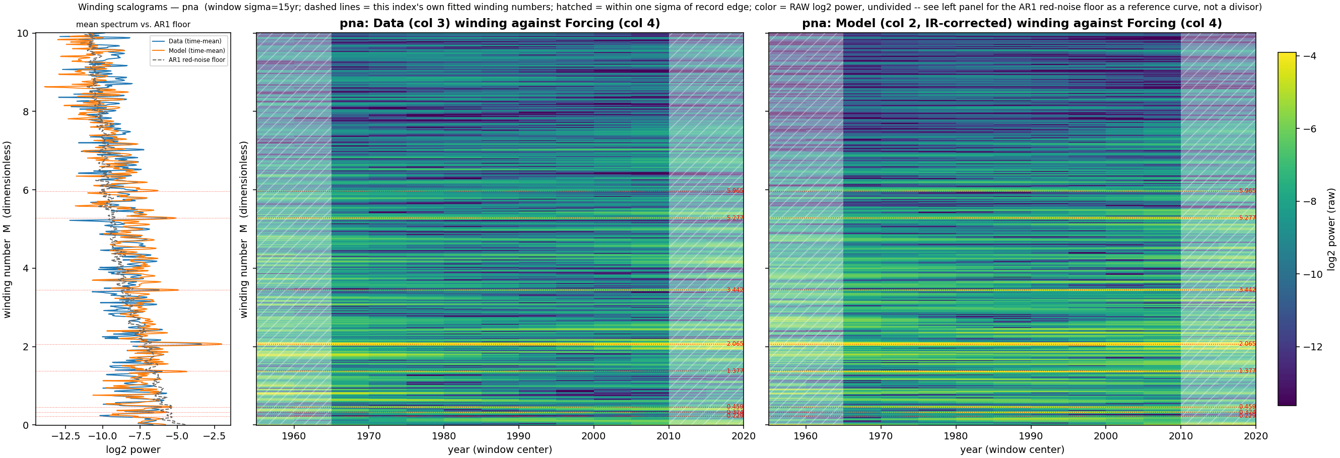
YET, if we apply the universal latent manifold identified via LTE analysis, and invoke a winding scalogram with respect to the data, we find strong continuous ridges indicating a stationary non-autonomous modulation is occurring and is likely causing the PNA cycles. Shown below is the winding scalogram, with the bright yellow indicating integer windings of the fundamental winding at 0.2065, the strongest being of the fundamental (compare this to a strong for the Baltic MSL and SSL)
The physical realization of this is the excellent cross-validated fit using the LTE mapping described in Mathematical Geoenergy, Chapter 121 shown below. The region from 1950 to 2001 was used for training, and the region after 2016 was used for predictive tuning, i.e. training produced a multiple regressed set of coefficients that projected into the future based on the manifold. After the training completed, the out-of-band interval shown by the dashed line below was used as a predictive test (the classic train/validate/test CV approach).
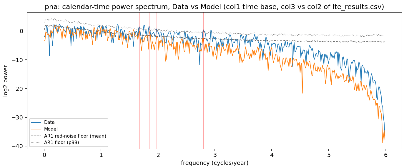
The test interval does show a drop in correlation but that can be expected given the erratic nature of the PNA cycle. This is a cyclic pattern that has eluded climate scientists essentially forever, as it barely exceeds red noise in its power spectrum (right). Yet a handful of winding transformations (with one strong winding, see below) about the manifold, identified by the winding spectrogram, and fitted to the PNA data is able to map the pattern more than good enough to pass a crucial cross-validation test. This is not just predicting past 10 days (as the quote at the top of this post claims), but potentially for years.
How can that be? In other words, how can this have gone unnoticed over decades of analysis? To understand that fully, consider that this LTE formulation falls in the same category as Mach-Zehnder modulation2. The complexity of the transfer function in M-Z modulation is of sufficient nonlinearity that it has been used as a practical encryption scheme for analog signals3. The gist of this is that if you don’t know the decryption key, you don’t have a chance of decoding a M-Z encoded signal. But if you do have it, the decryption is concise and fast. There are infinitely many encryption keys possible, so it’s not practical to enumerate and try to discover their value in any systematic way. Applying NVIDIA-powered AI algorithms are of no help here either, as the search space is much too large to explore.
But remember that in our context, nature can narrow down the encryption key possibilities — there aren’t infinitely many to choose from, but instead the ones that make sense are governed by physics and so can be formulated and straightforwardly evaluated. That’s why the LOD-calibrated (from a set of tidal factors) manifold worked — it was essentially the first one that I considered4 and have been tweaking for some time, long before the advent of convenient LLM tools. It also makes sense in the case of PNA — the geospatial dynamics of the tri-pole pressure pattern should remind one of amphidromic tidal patterns in the oceans (see right). These are due to the faster conventional diurnal tides, but they hint at how the long-period tidal factors impact the massive inertia of the subsurface waters — as that’s where the source and sink for tropospheric heat resides.
So that explains why this research may succeed — the answer was never really overlooked nor hidden in conventional signal processing artifacts. It was actually uncovered by an educated guess at what the decryption key was. All these ocean indices are falling like dominoes — NINO4, AMO, PDO, any MSL site, etc can be modelled with the LOD-calibrated manifold. Will show the Southern Annular Mode index next go round.
Pukite, Paul. “Nonlinear Differential Equations with external forcing.” ICLR 2020 Workshop on Integration of Deep Neural Models and Differential Equations. openreview.net/pdf?id=XqOseg0L9Q↩︎
Takiguchi, K. and Ishihara, W., “Encryption of 300 GHz-band wireless signal using optical vector modulator-type encoder”, in Society of Photo-Optical Instrumentation Engineers (SPIE) Conference Series, 2026, vol. 13895, Art. no. 1389506. doi:10.1117/12.3078963; Vaidman, L. (1995). “Cryptographic scheme based on a Mach-Zehnder interferometer.” Physical Review Letters, 75(18), 3206. Physical Review Letters. ↩︎
AMO is measured in the north Atlantic, and influenced by an annual cycle — at a latitude that is inclined more to the Sun in the summer (peak declination is at summer solstice) than winter.
ENSO resides on the equator, subject to the topological constraints of that boundary condition. It therefore gets influenced by a northern hemisphere cycle and a southern hemisphere cycle. This turns into a semi-annual cycle.
Mechanical torques to the Earth’s rotation are measured by deviations in the Earth’s length-of-day (LOD) — see the time-series below1. There is a clear annual and semi-annual cycle apparent as evidenced in the top panel, and also a gradual multi-decadal variation. Much stronger underlying this variation is a steady lunar tidal cycling, see bottom panel, where it is most easily revealed by taking the time-derivative of LOD — a real torque, or instantaneous acceleration. This decomposes to fundamental Mf,Mm, and Mf ‘ tidal cycles, with the Mf and Mm interfering to create an 8.848y perigean cycle, and the Mf and Mf ‘ interfering to create an 18.6 year nodal cycle. These beat envelopes can clearly be seen in the lower panel, along with occasional disturbances related to El Nino events (e.g. very strong 1983, 1988, 1992, very strong 1998, 2008)
A geophysical ansatz cooperatively linking LOD changes to climate cycles such as El Nino (ENSO), lies in the annual and semi-annual impulses that likely reinforce the instantaneous tidal torque that occurs at that time2. The premise is that torque over an impulse duration leads to an incremental level shift in LOD and that generates an internal (i.e. hidden) latent forcing manifold for the ocean’s fluid dynamics. This is particularly sensitive along the subsurface thermocline, where effective gravity is reduced.
Consider the northern Atlantic first. The forcing manifold is generated via a convolution (i.e. essentially integrated) of the annual impulses with the tidal torque at that instance. The strongest constituent tidal factor Mf shown below generates a ~3.8 year cycle over time as it alternates between reinforcing or canceling in sign. The value of 3.8 is determined via modulo arithmetic, 365.242/13.66 mod 1 ~ 3.8. Similarly, the Mf ‘ and Mm lead to ~4.8 and 3.9 year cycles.
These are the strongest cycles by amplitude, but due to a fortuitous commensurate alignment with the annual signal, the Mt tidal has a significant impact on the shape of the manifold. The fact that 40 of the 9.133 Mt tidal cycles fit almost precisely into a year means that constructive interferences gradually accumulate over a 60-year period and then change sign and decrement over the next 60-year interval. This rides on top of the faster 3.8, 3.9, and 4.8 year cycles creating an erratic staircase as shown below. There is a behavior known in fluid dynamics called a devil’s staircase which likely has a meaningful relationship to this form.3
But this is just the manifold, a forcing that can be considered as almost a phase envelope — we are not yet seeing the oceanic basin’s response to his forcing. That’s why considering it a phase makes intuitive sense, as the response may simply be a sine wave acting on this phase, i.e. A sin (k*phase)+ B cos(k*phase) where k is a constant. This is where the fluid dynamics mathematics of Laplace’s Tidal Equations (LTE) and LTE modulation fits in, as described in detail in Chapter 12 of Mathematical Geoenergy2. That text provides a non-intuitive grounding to what until now has a first-order physics explanation.
To get a feel for what this — in reality a non-linear response — involves computationally, consider the modulation/transfer function shown below:
That’s what it looks like with a k-modulation over the entire phase envelope, as it essentially doubles the frequency, changing the 120-year cycle to a 60-year cycle — not coincidentally the same period as the multidecadal period of the AMO.
Yet that 60-year cycle is only a single feature of the AMO, which is also characterized by wildly erratic fluctuations in value that almost obscure the multidecadal envelope. What actually works better as a model is if the shorter Mf steps on the staircase resolve to a complete single-period sinusoidal response, what in mathematical parlance is referred to a winding number of 1. The effective model thus becomes , where = phase, shown below for k = 1.55 and = 0.5. The phase slippage due to Mt causes the response to wander about zero over several decades.
The mapping to LOD remains largely intact through this as the 18.6 year and 8.85 year envelope is still clear. Note that a model of LOD is required to extrapolate before 1962, when the first LOD precision measurements were available.
The monthly and fortnightly remained near the same, but longer term tidal factors greater than 1 year in period had to be included (see bars in gray below), ostensibly to accommodate the drift in LOD estimated over the ~150 year time span of AMO.
The promise of the LOD-calibrated mathematical modeling further explains how the AMO itself may feed back into the LOD itself, as many have noted the multi-decadal variation in LOD resembles that of AMO5
The next step is to evaluate NINO34 (i.e. ENSO), lying along the equator. The distinction here is that the annual impulse, used for AMO, must be converted to a semi-annual impulse (one positive [+] excursion alternating with one negative [-] excursion). Note that the semi-annual nature destroys the constructive interference of the Mt ordinal, which created the 120-year staircase. Instead, we have a strong ~3.8yr up and down devil’s staircase manifold. So, we can evaluate the following chart — middle left shows the estimated manifold and middle right shows the sin(k) LTE modulation applied to achieve the top panel left model fit in red.
The semi-annual forcing is doing as predicted — it breaks the Mt-driven secular 120-year build-up and replaces it with a bounded, alternating step manifold that behaves like an ENSO-scale oscillator rather than an AMO staircase.
Top left: the red model tracks the broad phase/envelope of the blue NINO4 series well.
Top right: the scatter is clearly elongated along a positive slope, so the fit is not accidental. Some of the validation points are outside the regression set.
Middle left: this is the key result. The latent forcing is no longer a undulating staircase; it sits on recurring discrete bands, mostly between about -1.6 and -0.3, with occasional jumps toward 0 to +0.3. That is exactly the signature of the alternating +/- semi-annual impulse: an up/down “devil’s staircase” rather than constructive accumulation.
Middle right: the red sin(k) modulation overlays the dominant blue bands fairly well, especially on the main latent levels, so the modulation is using the tightened manifold. It occasionally underrepresents rare extremes.
Bottom left: the 50-month running correlation is usually high (~0.6–0.9) but drops down in the cross-validation interval. This could mean that the response is intermittently organized rather than uniformly phase-locked.
Bottom right: the PSD match is strongest at the low-order peaks; model and data line up well at the main maxima, while the data keeps more high-frequency power than the model. So the semi-annual latent structure captures the core resonant bands, but not all of ENSO’s fast variance.
Bottom line: this figure supports the idea that for equatorial ENSO/NINO4, the correct latent driver is a semi-annual alternating pulse, yielding a compact, oscillatory ~3.8-year staircase manifold instead of the long constructive Mt staircase used for AMO/NAO. The manifold looks physically coherent and the modulation is plausible, but the weak validation window says the current mapping is still less robust and more regime-dependent than the AMO case.
An amazing concordance is that the k = 1.55 and = 0.5 are essentially the same for ENSO as for AMO, indicating this is likely a common-mode temporal response. It’s possible that these are related to Arnold tongue resonances6 In terms of plausibility and parsimony of these preliminary results, note how modest the Arnold winding is on the middle right panel (winding=2 suggests one winding for northern hemisphere and one for southern hemisphere) which may be related to the topological time reversal symmetry rules of the equatorial region7. If the equatorial latent manifold were showing many wraps, that would look more like a flexible fitting device; a winding of about 2 is close to the minimal nontrivial topology you would expect for an equatorial interface problem.
The reason this is plausible is that the equator is special: the Coriolis sign flips across it, so north and south contributions should enter with opposite handedness rather than accumulate into the same long constructive winding. In that setting, a two-sheet / two-turn organization — one branch associated with the northern side, one with the southern side — is a natural first-order picture. That the interpretation of the middle-right panel: the modulation is not over-twisted; it is just wrapped enough to separate the main latent bands and recover the top-left fit. That is also consistent with the Delplace/Marston style topological view of the equator as an interface where symmetry strongly constrains admissible structure.
On parsimony, this is good news. The model already uses a semi-annual sign-alternating impulse, which by itself suppresses the Mt constructive staircase and forces a bounded oscillatory manifold. Once that choice is made, a small winding number is the simplest way to map that latent staircase into ENSO-like oscillation. So, the topology is doing real work without needing a large number of wraps, a high-order phase map, or a visually baroque modulation.
So, what would one expect for PDO? Since it inhabits the northern Pacific, one would expect an annual impulse. Borrowing the parameters from AMO, it fits the pattern cleanly with a sharply delineated LTE modulation. Note that even though PDO is considered to have some of the character of ENSO, the fact that the k = 1.55 and = 0.5 parameters are again the same, indicates the common-mode behavior of these climate indices.
NAO — North Atlantic Oscillation
It does also work for coastal mean sea level (MSL) tidal stations : Ratan, Sweden
IOD East (Indian Ocean Dipole) — Letting it free fit drove the Mt amplitude to a lower value. This indicated that the 120-year cycle was weaker, so adjusted this by adding a partial semi-annual component of -2/3 the amplitude of the annual impulse. The Indian Ocean straddles the equator but Asia to the north really clips off that lobe.
TNA (Tropical North Atlantic) — has characteristics of AMO
TSA (Tropical South Atlantic). Is this more like ENSO?
Set of west coast MSL sites
All the tidal factors were allowed to vary as that was the easiest way to optimize and escape local minimum, but the distribution of weightings remained roughly the same in the 9 cases fitted above. Since the k and values also stayed even tighter, it’s possible that the cyclic fingerprint of each index is a combination of slightly different tidal factor contributions and the balance between annual and semi-annual impulses for that geospatial location. In fact, it might turn out that a more efficient fitting process is to start from a Bayesian-average tidal factor configuration instead of from the LOD calibration. This would reinforce the idea that this is truly a commo-mode behavior.
Eye-chart of tidal factor weightings top row: NINO4, AMO, PDO middle: NAO, IOD, TNA bottom : Ratan, TSA, West Coasr
Tidal Amplitude Spectrum (Complete)
Tidal Amplitude Spectrum
Complete dataset with all 32 periods from each directory
Dataset Summary: All 9 directories (nino4, amo, pdo, nao, iode, tsa, tna, 88, wcoast)
with identical period structure. Periods > 365 days shown in gray background.
Loading complete dataset…
Period (days)
nino4
amo
pdo
nao
iode
tsa
tna
88
wcoast
27.322
0.00766
-0.00284
0.01103
-0.00969
-0.00739
0.00909
0.01308
-0.01308
-0.00607
27.212
-0.00962
0.00230
0.00945
0.00914
0.00161
0.01352
0.00803
0.01839
0.01288
1095.175
-0.01868
0.02688
0.01759
0.03896
0.01075
-0.00192
0.02392
0.00838
-0.01754
13.633
0.12949
0.13477
0.12649
0.12599
0.12452
0.11459
0.12611
0.12162
0.12957
13.661
-0.32865
-0.32034
-0.31731
-0.31815
0.31652
0.32392
-0.33320
-0.27666
-0.33224
13.606
0.00260
0.00416
0.01435
0.00698
0.01250
0.00842
0.00101
0.00438
-0.00091
27.555
0.09385
0.10842
0.10792
0.12372
0.08670
0.07237
0.09408
0.09734
0.07357
13.777
0.01859
-0.00784
-0.02674
-0.02157
0.02300
0.03332
0.03225
0.01120
0.01611
6793.476
0.02504
0.02121
0.01668
0.02042
0.00315
-0.00828
0.02291
0.01651
-0.01100
1616.303
0.01552
0.02624
0.01918
0.03517
0.01843
-0.02135
-0.01741
0.01525
0.01810
31.812
0.01048
0.03055
0.00594
0.03619
0.01400
0.02974
0.01963
0.02012
0.01433
1305.660
0.01901
0.03236
-0.03170
0.03310
0.01787
-0.00542
0.03654
0.03207
0.02456
27.443
0.00652
0.01137
0.02500
0.01133
0.00575
0.00662
-0.01227
0.02264
0.01039
27.667
0.00577
-0.00979
-0.01894
-0.00478
0.00373
-0.00881
0.00596
-0.01864
0.00804
2190.350
-0.00067
-0.00377
-0.01081
-0.00453
0.01231
0.02257
0.00866
-0.00940
0.00176
26.985
-0.00403
-0.01943
-0.02923
-0.02621
0.01077
-0.01067
-0.02716
-0.03490
-0.00994
6167.207
0.02099
0.02246
0.01566
0.02475
0.00688
-0.00498
0.02517
0.02452
0.02442
-3232.605
-3.23261
-3.23261
-3.23261
-3.23261
-3.23261
-3.23261
-3.23261
-3.23261
-3.23261
-2120.909
-2.12091
-2.12091
-2.12091
-2.12091
-2.12091
-2.12091
-2.12091
-2.12091
-2.12091
9.133
-0.09976
-0.09955
-0.09969
-0.09937
0.08648
0.08693
-0.09904
-0.10074
-0.10239
9.121
0.03385
0.03216
0.03412
0.03067
0.02595
0.03089
0.03352
0.02750
-0.03579
9.108
0.00603
0.00756
-0.01066
0.01400
0.01007
-0.01007
0.00698
0.01054
-0.01824
3396.738
0.02810
0.02401
0.01968
0.02000
0.00397
-0.02470
0.03562
0.02245
0.03287
1656.320
0.02340
0.01163
0.00986
0.00633
0.03245
-0.01107
0.03341
0.00394
0.05237
9.557
0.03658
0.04203
0.04366
0.04931
0.03202
0.02256
0.04357
0.05432
0.05022
9.185
0.00346
-0.00769
-0.01111
-0.00180
-0.00351
0.01015
-0.01492
-0.00934
-0.00787
9.543
-0.05449
0.00000
0.00000
-0.01272
0.01353
0.03086
-0.02726
-0.05449
0.02336
7.088
-0.01554
-0.02351
-0.03860
-0.00661
0.00934
-0.00321
0.00462
-0.05186
0.03153
6.852
0.00726
0.01444
-0.01266
0.02624
0.00929
-0.00650
-0.01818
0.01203
0.01498
6.859
0.01970
0.01144
0.00828
0.01353
0.01679
0.00888
0.00510
-0.00622
0.01316
7.096
-0.00619
0.00846
0.01787
0.01701
0.00989
0.01929
0.00928
0.00468
0.00447
5.643
-0.00619
0.00846
0.01787
0.01701
0.00989
0.01929
0.00928
0.00468
0.00447
Note: Gray background indicates periods > 365 days (long periods). White background indicates periods ≤ 365 days (short periods).
Important: Values are amplitudes from the lt.exe.p JSON files. Negative values indicate phase differences.
Total entries: 32 periods × 9 directories = 288 amplitude values displayed.
The IOD-East and TSA, both south of the equator are close to the LOD composite
Is this the deeper physics?
Delplace, Marston, and Venaille showed that equatorial Kelvin and Yanai waves arise as topologically protected edge modes, associated with a bulk Chern number of 2 for the rotating shallow‑water Poincaré spectrum in (k,ω) space. Their result is an abstract existence theorem: it guarantees robust equatorial waves but does not specify how they are forced or parameterized in time for prediction. In contrast, the LTE manifold used here selects an equatorial standing mode consistent with that topology and embeds it in a time‑domain, lunisolar‑forced framework, with explicit annual impulses and nonlinear modulation fitted directly to ENSO, AMO, and tide‑gauge records. In this sense, the LTE formulation provides a practical parameterization that connects the topological structure of equatorial waves to applied, data‑driven prediction in physical time.
From a dynamical‑systems perspective, the LTE manifold treats ENSO and related indices as the response of a phase‑locked forced oscillator, living in a low‑dimensional latent space and driven by a small set of quasi‑periodic forcings (lunisolar tides plus an annual impulse). In the language of nonlinear dynamics, this is an explicitly parameterized instance of mode locking on a torus (Arnold tongues, Devil’s staircase, Farey‑ordered p:q plateaus), while in the language of topological fluids it corresponds to driving a protected equatorial edge mode (Kelvin/Yanai‑like) selected by the bulk Chern structure of the rotating shallow‑water system. In modern ML terms, the construction is a physics‑informed analogue of SINDy/KAN latent‑manifold models8: a shared, low‑dimensional latent driver is specified a priori, and simple nonlinear mappings (amplitude, phase, sinusoidal folding) are fitted to map that latent trajectory into many observed time series, providing an interpretable bridge between abstract topological theory and data‑driven prediction.
There is enough here for ML to extend, but the proviso is that the detailed LOD forcing must be applied -- I don't think it will work unless enough of the constituent tidal factors (ranked strongest to weakest) are included. The complexity of ENSO or AMO is a result of a Mach-Zehnder-like encryption of an already multi-constituent cycle - that's essentially impossible to decode without a valid manifold key.
Mathematical Geoenergy, Pukite, P.R. et al, (Wiley/AGU, 2019) ↩︎
Marcus, S. L., 2016: Does an Intrinsic Source Generate a Shared Low-Frequency Signature in Earth’s Climate and Rotation Rate?. Earth Interact., 20, 1–14, https://doi.org/10.1175/EI-D-15-0014.1.. ↩︎
The behavior of complex systems, particularly in fluid dynamics, is traditionally described by high-dimensional systems of equations like the Navier-Stokes equations. While providing practical applications as is, these models can obscure the underlying, simplified mechanisms at play. It is notable that ocean modeling already incorporates dimensionality reduction built in, such as through Laplace’s Tidal Equations (LTE), which is a reduced-order formulation of the Navier-Stokes equations. Furthermore, the topological containment of phenomena like ENSO and QBO within the equatorial toroid , and the ability to further reduce LTE in this confined topology as described in the context of our text Mathematical Geoenergy underscore the inherent low-dimensional nature of dominant geophysical processes. The concept of hidden latent manifolds posits that the true, observed dynamics of a system do not occupy the entire high-dimensional phase space, but rather evolve on a much lower-dimensional geometric structure—a manifold layer—where the system’s effective degrees of freedom reside. This may also help explain the seeming paradox of theinverse energy cascade, whereby order in fluid structures seems to maintain as the waves become progressively larger, as nonlinear interactions accumulate energy transferring from smaller scales.
Discovering these latent structures from noisy, observational data is the central challenge in state-of-the-art fluid dynamics. Enter the Sparse Identification of Nonlinear Dynamics (SINDy) algorithm, pioneered by Brunton et al. . SINDy is an equation-discovery framework designed to identify a sparse set of nonlinear terms that describe the evolution of the system on this low-dimensional manifold. Instead of testing all possible combinations of basis functions, SINDy uses a penalized regression technique (like LASSO) to enforce sparsity, effectively winnowing down the possibilities to find the most parsimonious, yet physically meaningful, governing differential equations. The result is a simple, interpretable model that captures the essential physics—the fingerprint of the latent manifold. The SINDy concept is not that difficult an algorithm to apply as a decent Python library is available for use, and I have evaluated it as described here.
Applying this methodology to Earth system dynamics, particularly the seemingly noisy, erratic, and perhaps chaotic time series of sea-level variation and climate index variability, reveals profound simplicity beneath the complexity. The high-dimensional output of climate models or raw observations can be projected onto a model framework driven by remarkably few physical processes. Specifically, as shown in analysis targeting the structure of these time series, the dynamics can be cross-validated by the interaction of two fundamental drivers: a forced gravitational tide and an annual impulse.
The presence of the forced gravitational tide accounts for the regular, high-frequency, and predictable components of the dynamics. The annual impulse, meanwhile, serves as the seasonal forcing function, representing the integrated effect of large-scale thermal and atmospheric cycles that reset annually. The success of this sparse, two-component model—where the interaction of these two elements is sufficient to capture the observed dynamics—serves as the ultimate validation of the latent manifold concept. The gravitational tides with the integrated annual impulse are the discovered, low-dimensional degrees of freedom, and the ability of their coupled solution to successfully cross-validate to the observed, high-fidelity dynamics confirms that the complex, high-dimensional reality of sea-level and climate variability emerges from this simple, sparse, and interpretable set of latent governing principles. This provides a powerful, physics-constrained approach to prediction and understanding, moving beyond descriptive models toward true dynamical discovery.
Crucially, this analysis does not use the SINDy algorithm, but a much more basic multiple linear regression (MLR) algorithm predecessor, which I anticipate being adapted to SINDy as the model is further refined. Part of the rationale for doing this is to maintain a deep understanding of the mathematics, as well as providing cross-checking and thus avoiding the perils of over-fitting, which is the bane of neural network models.
Also read this intro level on tidal modeling, which may form the fundamental foundation for the latent manifold: https://pukpr.github.io/examples/warne_intro.html. The coastal station at Wardemunde in Germany along the Baltic sea provided a long unbroken interval of sea-level readings which was used to calibrate the hidden latent manifold that in turn served as a starting point for all the other models. Not every model works as well as the majority — see Pensacola for a sea-level site and and IOD or TNA for climate indices, but these are equally valuable for understanding limitations (and providing a sanity check against an accidental degeneracy in the model fitting process) . The use of SINDy in the future will provide additional functionality such as regularization that will find an optimal common-mode latent layer,.
The last set of cross-validation results are based on training of held-out data for intervals outside of 0.6-0.8 (i.e. training on t<0.6 and t>0.8 of the data, which extends from t=0.0 to t=1.0 normalized). This post considers training on intervals outside of 0.3-0.6 — a narrower training interval and correspondingly wider test interval.
Each fitted model result shows the cross-validation results based on training of held-out data — i.e. training on only the intervals outside of 0.6-0.8 (i.e. training on t<0.6 and t>0.8 of the data, which extends from t=0.0 to t=1.0 normalized). The best results are for time-series that have 100 years or more worth of monthly data, so the held-out data is typically 20 years. There is no selection bias trickery here, as this is a collection of independent sites and nothing in the MLR fitting process is specific to an individual time-series. In the following, the collection of results starts with the Stockholm site in Sweden, keeping in mind that the dashed line in the charts indicates the test or validation interval.
I was recently in Stockholm, and this is a photo pointed toward the location of the measurement station, about 4000 feet away labeled by the marker on the right below:
“New research shows the natural variability in climate data can cause AI models to struggle at predicting local temperature and rainfall.” … “While deep learning has become increasingly popular for emulation, few studies have explored whether these models perform better than tried-and-true approaches. The MIT researchers performed such a study. They compared a traditional technique called linear pattern scaling (LPS) with a deep-learning model using a common benchmark dataset for evaluating climate emulators. Their results showed that LPS outperformed deep-learning models on predicting nearly all parameters they tested, including temperature and precipitation.“
Machine learning and other AI approaches such as symbolic regression will figure out that natural climate variability can be done using multiple linear regression (MLR) with cross-validation (CV), which is an outgrowth or extension of linear pattern scaling (LPS).
“When this was initially created on 9/1/2025, there were 3000 CV results on time-series that averaged around 100 years (~1200 monthly readings/set) so over 3 million data points“
In this NINO34 (ENSO) model, the test CV interval is shown as a dashed region
I developed this github model repository to make it easy to compare many different data sets, much better than using an image repository such as ImageShack.
There are about 130 sea-level height monitoring stations in the sites, which is relevant considering how much natural climate variation a la ENSO has an impact on monthly mean SLH measurements. See this paper Observing ENSO-modulated tides from space
“In this paper, we successfully quantify the influences of ENSO on tides from multi-satellite altimeters through a revised harmonic analysis (RHA) model which directly builds ENSO forcing into the basic functions of CHA. To eliminate mathematical artifacts caused by over-fitting, Lasso regularization is applied in the RHA model to replace widely-used ordinary least squares. “
Someone on Twitter suggested that tidal models are not understood “The tides connection to the moon should be revised.”. Unrolled thread after the “Read more” break
The machine learning community needs to be let loose on this data. The tidal forcing is a latent or hidden layer that ML models such a SINDy, KAN, and others could easily handle. I don't use ML other than to fit the models with known tidal factors – ManMachineLearning so far.
A climate teleconnection is understood as one behavior impacting another — for example NINOx => AMO, meaning the Pacific ocean ENSO impacting the Atlantic ocean AMO via a remote (i.e. tele) connectiion. On the other hand, a common-mode behavior is a result of a shared underlying cause impacting a response in a uniquely parameterized fashion — for example NINOx = g(F(t), {n1, n2, n3, ...}) and AMO = g(F(t), {a1, a2, a3, ...}), where the n's are a set of constant parameters for NINOx and the a's are for AMO.
In this formulation F(t) is a forcing and g() is a transformation. Perhaps the best example of a common-mode response to a forcing is in the regional tidal response in local sea-level height (SLH). Obviously, the lunisolar forcing is a common mode in different regions and subtle variations in the parametric responses is required to model SLH uniquely. Once the parameters are known, one can make practical predictions (subject to recalibration as necessary).
By applying an annual impulse sample-and-hold on a common-mode basis set of tidal factors, a wide range of climate indices can be modeled and cross-validated. Whether it is a biennial impulse or annual impulse, the slowly modulating envelope is roughly the same, thus models of multidecadal indices such as AMO and PDO show similar skill — with cross validation results evaluated here for a biennial impulse. Now we will evaluate for annual impulse.