The ocean heat content continues to increase and perhaps accelerate [1], as expected due to global warming. In an earlier post, I analyzed the case of the “missing heat”, which wasn’t missing after all, but the result of the significant heat sinking characteristics of the oceans [2].

The objective is to create a simple model which tracks the transient growth as shown in the recent paper by Balmaseda, Trenberth, and Källén (BTK)[1] and described in Figure 1 below

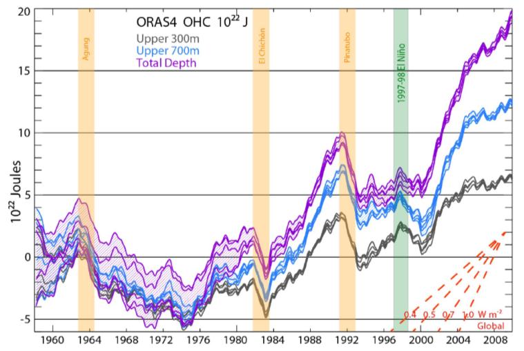Figure 1: Ocean Heat Content from BTK [1] (source)

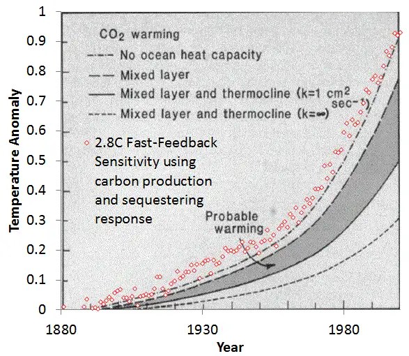
We will assume a diffusive flow of heat as described in James Hansen’s 1981 paper [2]. In general  the diffusion of heat is qualitatively playing out according to the way Fick’s law would apply to a heat sink. Hansen also volunteered an effective diffusion that should apply, set to the nice round number of 1 cm^2/second.

In the following we provide a mathematical explanation which works its way from first principles to come up with an uncertainty-quantified formulation. After that we present a first-order sanity check to the approximation.

Solution

We have three depths that we are looking at for heat accumulation (in addition to a surface layer which gives only a sea-surface temperature or SST). These are given as depths to 300 meters, to 700 meters, and down to infinity (or 2000 meters from another source), as charted on Figure 1.

We assume that excess heat (mostly infrared) is injected through the ocean’s surface and works its way down through the depths by an effective diffusion coefficient.  The kernel transient solution to the planar heat equation is this:

$$\Delta T(x,t) = \frac{c}{\sqrt{D_i t}} \exp{\frac{-x^2}{D_i t}} $$
where D_i is the diffusion coefficient, and x is the depth (note that often a value of 2D instead of D is used depending on the definition of the random walk).  The delta temperature is related to a thermal energy or heat through the heat capacity of salt water, which we assume to be constant through the layers. Any scaling is accommodated by the prefactor, c

The first level of uncertainty is a maximum entropy prior (MaxEnt) that we apply to the diffusion coefficient to approximate the various pathways that heat can follow downward.  For example, some of the flow will be by eddy diffusion and other paths by conventional vertical mixing diffusion.  If we apply a maximum entropy probability density function, assuming only a mean value for the diffusion coefficient:
$$ p(D_i) = \frac{1}{D} e^{\frac{-D_i}{D}} $$

then we get this formulation:
$$\Delta T(t|x) = \frac{c}{\sqrt{D t}} e^{\frac{-x}{\sqrt{D t}}} (1 + \frac{x}{\sqrt{D t}})$$

The next uncertainty is in capturing the heat content for a layer. The incremental heat across a layer, L, we can approximate as
$$ \int { \Delta T(t|x) p(x) dx}  = \int { \Delta T(t|x) e^{\frac{-x}{L}} dx} $$

Which gives as the excess heat response the following concise equation.
$$ I(t) = \frac{ \frac{\sqrt{Dt}}{L} + 2 }{(\frac{\sqrt{Dt}}{L} + 1)^2}$$

This is also the response to a delta forcing impulse, but for a realistic situation where a growing aCO2 forces the response (explained in the previous post), we simply apply a convolution of the thermal stimulus with the thermal response.  The temporal profile of the increasing aCO2 generates a growing thermal forcing function.

$$ R(t) = F(t) \otimes I(t) = \int_0^t { F(\tau) I(t-\tau) d\tau} $$
If the thermal stimulus is a linearly growing heat flux, which roughly matches the GHG forcing function (see Figure 7 in the previous post)
 $$ F(t) = k \cdot (t-t_0) $$
then assuming a starting point t_0=0.
$$ R(t)/k = \frac{2 L}{3} {(D t)}^{1.5}- L^2 D t+2 L^3 \sqrt{D t}-2 L^4 \ln(\frac{\sqrt{D t}+L}{L})) $$

A good approximation is to assume the thermal forcing function started kicking in about 50 years ago, circa1960. We can then plot the equation for various values of the layer thickness, L, and a value of D of 3 cm^2/s.

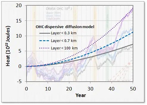Figure 2 : Thermal Dispersive Diffusion Model applied to the OHC data

Another view of the OHC includes the thermal mass of the non-ocean regions (see Figure 3). This data appears smoothed in comparison to the raw data of Figure 2.

Figure 3 :  Alternate view of growing ocean heat content. This also includes non-ocean.

In the latter figure, the agreement with the uncertainty-quantified theory is more striking. A single parameter, Hansen’s effective diffusion coefficient D, along with the inferred external thermal forcing function is able to reproduce the temporal profile accurately.

The strength of this modeling approach is to lean on the maximum entropy principle to fill in the missing gaps where the variability in the numbers are uncertain.  In this case, the diffusion and ocean depths hold the uncertainty, and we use first-order phyiscs to do the rest.

Sanity Check

The following is a sanity check for the above formulation; providing essentially a homework assignment that a physics professor would hand out in class.

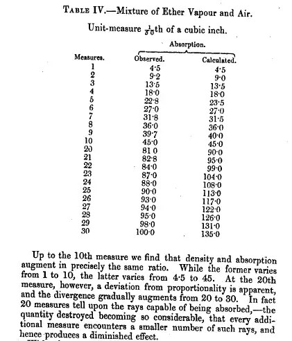
An application of Fick’’s Law is to approximate the amount of material that has diffused (with thermal diffusion coefficient D) at least a certain distance, x, over a time duration, t, by

$$ e^{\frac{-x}{\sqrt{Dt}}}= \frac{Q}{Q_0}$$

• For greater than 300 meters, Q/Q_0 is 13.5/20 read from Figure 1.
• For greater than 700 meters, Q/Q_0 is 7.5/20

Where Q_0=20 is the baseline for the total heat measured over all depths (i.e. between x=0 and x=infinite depth) reached at the current time. No heat will diffuse to infinite depths so at that point Q/Q_0 is 0/20.

First, we can check to see how close the value of L=sqrt(Dt) scales, by fitting the Q/Q_0 ratio at each depth..

• For x=300 meters, we get L=763
• For x=700 meters, we get L=713

These two are close enough to maintaining invariance that the Fick’’s law scaling relation holds and we can infer that the flow is by an effective diffusion, just as was surmised by Hansen et al in 1981.

We then use an average elapsed diffusion time of t=40 years and assume an average diffusion depth of 740, and D comes out to 4.5 cm^2/s.

Hansen in 1981 [2] used an estimated value of diffusion of 1 cm^2/s, which is within an order of magnitude of 4.5 cm^2/s

This is a scratch attempt at an approximate solution to the more general solution, which is the equivalent of generating an impulse function in the past and watching that evolve. The general solution which we formulated earlier involves a modulated forcing function and we compute the convolution against the thermal impulse response (i.e. Green’s function) and compare that against Figure 1 and Figure 2, and the full temporal profile.

Discussion

Reading Hansen and looking at the BTK paper’s results, we should note that nothing looks out of the ordinary for the OHC trending if we compare it to what conventional thermal physics would predict. The total heat absorbed by the ocean is within  range of that expected by a 3C doubling sensitivity. BTK has done the important step in determining the amount of total heat absorbed, which allows us to estimate the effective diffusion coefficient by evaluating how the heat contents modulate with depth.We add a maximum uncertainty modifier to the coefficient to model the disorder in diffusivity (some of it eddy diffusivity, some vertical, etc) and that allows us to match the temporal profile accurately.

References

 EDITED 

More data from the NOAA site using the same fit. Levitus et al [3] apply an alternative characterization to the above. I apply the same model as dashed green line.

Figure 4 : From the NOAA site, with the same model http://www.nodc.noaa.gov/OC5/3M_HEAT_CONTENT/

And here is a plot of OHC using the effective forcing described by Hansen [4]. Instead of using a ramp forcing function which gives the analytical result of Figure 2, a realistic forcing (which takes into account perturbations due to volcanic events) is numerically convolved with the diffusive response function, I(t).

Figure 5: Numerical convolution of effective forcing (lower left) is convolved with the diffusive transfer function to give the response (upper right).  The three curves are < 300 m,  < 700 m, and < 2000 m.

Note that the volcanic disturbances are clearly visible in the response, although they do not show as sharp a transient decrease after the events, perhaps half of what Figure 1 shows. The suppression due to the 1997-1998 El Nino is also not observable, but that of course is not a effective forcing and so won’t appear.

Often both skeptics and non-skeptics of AGW will suggest that climate models and their simulations are becoming too unwieldy to handle.  Stochastic models of the climate are always an option to consider, as Marston points out in his paper “Looking for new problems to solve? Consider the climate“, where he recommended to

“look at the sort of question a statistical description of the climate system would be expected to answer” [5] . 

It is no wonder that applying stochasticity is one of the grand challenges in science. In the past few years, DARPA put together a list of 23 mathematical challenges inspired by Hilbert’s original list. Several of them feature large scale problems which would benefit from the stochastic angle that both Marston and David Mumford [4] have recommended:

• Mathematical Challenge 3: Capture and Harness Stochasticity in Nature
  Address David Mumford’s call for new mathematics for the 21st century. Develop methods that capture persistence in stochastic environments.  
• Mathematical Challenge 4: 21st Century FluidsClassical fluid dynamics and the Navier-Stokes Equation were extraordinarily successful in obtaining quantitative understanding of shock waves, turbulence and solitons, but new methods are needed to tackle complex fluids such as foams, suspensions, gels and liquid crystals.
• Mathematical Challenge 7: Occam’s Razor in Many Dimensions
  As data collection increases can we “do more with less” by finding lower bounds for sensing complexity in systems? This is related to questions about entropy maximization algorithms.
• Mathematical Challenge 20: Computation at Scale
  How can we develop asymptotics for a world with massively many degrees of freedom?

The common theme is one of reducing complexity, which is often at odds with the mindset of those convinced that only more detailed computations of complex models will accurately represent a system.

A representative phenomena of what stochastic processes are all about is the carbon cycle and the sequestering of CO2. Much work has gone into developing box models with various pathways leading to sequestering of industrial CO2. The response curve according to the BERN model [7] is series of damped exponentials showing the long term sequestering. Yet, by a more direct statistical interpretation of what is involved in the process of CO2 sequestration, we can model the adjustment time of CO2 decay by a dispersive diffusional model derived via maximum entropy principles.

$$ I(t) = \frac{1}{1+\sqrt{t/\tau}} $$

Figure 1 : Impulse response of atmospheric CO2 concentration due to excess carbon emission.

A main tenet of the AGW theory presupposes the evolution of excess CO2. The essential carbon-cycle physics says that the changing CO2 is naturally governed by a base level which changes with ambient temperature, but with an additional impulse response governed by a carbon stimulus, either natural (volcano) or artificial (man-made carbon). The latter process is described by a convolution, one of the bread and butter techniques of climate scientists:

$$CO_2(t,T) = CO_2(0,T) + \kappa \int_0^t C(\tau) I(t-\tau) d\tau $$

With the impulse response of Figure 1 convolved against the historical carbon outputs as archived at the CO2 Information Analysis Center, it matches the measured CO2 from the KNMI Climate Explorer with the following agreement:

Figure 2 : CO2 impulse response convolution

The match to the CO2 measurements is very good after the year 1900. No inexplicable loss of carbon to be seen. This is all explainable by diffusion kinetics into sequestration sites. Diffusional physics is so well understood that it is no longer arguable.

If on the other hand, you do this analysis incorrectly and use a naive damped exponential response ala Segalstad [1] and Salby [unpublished] and other contrarian climate scientists, you do end up apparently believing that half of the CO2 has gone missing. If that were indeed the case, this is what the response looks like, given the skeptics view of a short 6.5 year CO2 residence time:

Figure 3: Incorrect impulse response showing atmospheric CO2 deficit due to a short residence time. This is clearly not observed in the data

The obvious conclusion is that if you don’t do the statistical physics correctly, you end up with nonsense numbers.

Note that this does not contradict findings of the mainstream climate researchers, but it places our understanding on a potentially different footing, and one with potentially different insight.

Consider next the sensitivity of temperature to the log of atmospheric CO2. In 1863, Tyndall discovered the properties of CO2 and other gases via an experimental apparatus [3];he noticed that light radiation absorption was linear up to a point but beyond that the absorptive properties of the gas showed a diminishing effect:

Figure 4: Tyndall’s description of absorption of light rays by gases [6]

The non-linear nature derives from the logarithmic sensitivity of forcing to CO2 concentration. The way to understand this is to consider differential increases of gas concentration. In the test chamber experiment, this is just a differential increase in the length of the tube. The scattering cross-section is derived as a proportional increase to how much gas is already there so it integrates as the ratio of delta increase to the cumulative length of travel of the photon:

$$ \int_{L_0}^L \frac{dX}{X} = ln(\frac{L}{L_0}) \sim ln(\Delta{[CO_2]}) $$

So as the photon travels a length of tube, it gets progressively more difficult to increase the amount of scattering, not because it isn’t physically possible but because the photon has had a large probability of being intercepted already as it makes its way out of the atmosphere. That generates the logarithmic sensitivity.

Note that the lower bound of the integral has to exist to prevent a singularity in the proportional increase. To represent this another way, we can say that there is a minimum length at which the absorption cross-section occurs.

$$ \int_{0}^L \frac{dX}{X_0+X} = ln(\frac{X_0+L}{X_0}) \sim ln(1+\Delta{[CO_2]}) $$

The analogy to the test chamber is the height of the atmosphere. The excess CO2 that we emit from burning fossil fuels increases the concentration at the top of the atmosphere, and that increases the length of the travel of the outgoing IR photons, and the same logarithmic sensitivity results. This is incorrectly labeled as saturating behavior, instead of an asymptotic logarithmic behavior.

I haven’t seen this derived in this specific way but the math is high-school level integral calculus. The actual model used by Lacis and other climate scientists is to configure the cross-sections by compositing the atmosphere into layers or “slabs” and then propagating the interception of photons by CO2 by differential numerical calculations. In addition, there is a broadening of the spectral lines as concentration increases, contributing to the first order result of logarithmic sensitivity.  In general the more that the infrared parts of the photonic spectrum get trapped by CO2 and H20, the higher the temperature has to be to make up for the missing propagated wavelengths while not violating the earth’s strict steady-state incoming/outgoing energy balance.

To get a sense of this logarithmic climate sensitivity, the temperature response is shown to the below  right for a 3°C sensitivity to CO2 doubling, mapped against the BEST land-based temperature record. Observe that trending temperature shifts are already observed in the early 20th century.

Figure 5:  CO2 model applied to AGW via a log sensitivity and compared against the fast rsponse of BEST land-based records.

If we choose a 2.8°C sensitivity from Hansen’s 1981 paper [2] and compare the above model to Hansen’s projection, one can see that we are on the right track in duplicating his analysis.

Figure 6: Hansen’s original model projection circa 1981 [2] and the 2.8C model used here.

Perhaps the only real departure from the model is a warming around 1940 not accounted for by CO2.  But even this is likely due to a stochastic characteristic in the form of noise riding along with the trend.. This noise could be volcanic disruptions or ocean upwelling fluctuations of a random nature,  which only requires the property that upward excursions match downward.

So if we consider the difference between the green line model and blue line data below:

Figure 7: Plot used for regression analysis. Beyond 1900, the RMS error is less than 0.2 degrees

and take the model/data residuals over time, we get the following plot.

Figure 8: Regression difference between log sensitivity model and BEST data

Note that the yearly excursions never exceed about 0.2°C from the underlying trend.  The dotted line red curve above the solid blue residual curve is an Ornstein-Uhlenbeck model (red noise) of a yearly random walk with a reversion-to-the-mean drag that prevents fluctuations beyond approximately 0.2°C.  At this kind of scale and considering the Markov process which will allow short-term fluctuations in the tenths of a degree, the bump of increased temperature in the 1940’s is not a rare nor completely unlikely occurrence.

A red noise model on this scale can not accommodate both the short-term fluctuations and the large upward trend of the last 50 years. That is why the CO2-assisted warming is the true culprit, as evidenced by a completely stochastic analysis.

[EDIT]
Here is a sequence of red noise time series (of approximately 0.2°C RMS excursion) placed on top of an accelerating monotonically warming temperature profile (the no-noise accelerating profile is in the lower left panel). The actual profile is shown in the lower right panel. An averaging window of 30 years is placed on the profiles to give an indication of where plateaus, pauses, and apparent cooling can occur.

Figure 9: Hypothetical red noise series placed on an accelerating warming curve.

“Noise riders” are people that look at time series and read too much into each fluctuation. The temptation to place too much emphasis on recent readings is strong but ultimately misguided. Dead reckoning models are built-in as a human intuition mechanism but don’t serve us well in the face of noise.

The baseball analogy to the red noise of Figure 9 is the knuckle-ball pitcher. Being able to hit a knuckle-baller means that you have quick reflexes and an ability to suppress the dead reckoning urge.

R.A. Dickey’s Cy Young Knuckleball Pitch (SOURCE)

References

[6] Tyndall, John, 1861. On the Absorption and Radiation of Heat by Gases and Vapours, and on the Physical Connection of Radiation, Absorption, and Conduction. ‘Philosophical Magazine ser. 4, vol. 22, 169–94, 273–85.

[7] J. Golinski, “Parameters for tuning a simple carbon cycle model,” United Nations Framework Convention on Climate Change. [Online]. Available: http://unfccc.int/resource/brazil/carbon.html. [Accessed: 12-Mar-2013].

In terms of climate statistics, we always have more data than we know what to do with. The challenge is in reducing the data into meaningful bits of information which can be characterized and modeled succinctly.

So this is a case of where enough data exists that we can get an understanding of the spatial and temporal correlations of prevailing winds.

One source of data comes from measurements of winds at altitude, taken by jet airliners as part of their regular flight routes and then post-processed and analyzed[1]. This gives an indication of spatial correlation over a large dynamic range, stretching a little over three orders of magnitude.  Once collected, the post-processing involved applying an autocorrelation to the data over all spatial scales.  The power spectral density (PSD) is the Fourier transform of the autocorrelation, and that is shown in Figure 1 below, along with a suggested model achieving a good fit to the actual meridonal wind PSD.

Figure 1 : Zonal and Meridional wind speed PSD. The dashed line model fit works well apart from deviations near the noisy shorter wavelengths.

The chosen model is simply the PSD of an exponentially damped cosine autocorrelation (see [2] for examples in meteorology).

$$ C(x) = e^{-\alpha |x|} \cdot cos(\beta x) $$

The Fourier transform of this autocorrelation gives a PSD that is best described as a shifted Cauchy or Lorentzian profile.  In Figure 1, the shape is obvious as it shows a peak and then a concave-upward inflection following the peak.

$$ I(S_x) = \frac{\alpha}{(S_x-\beta)^2 + \alpha^2} $$

This specific profile is generated by a semi-Markovian process.  The “semi” part captures the periodic portion while the Markov contributes the memory for close-proximity coupling. Specifically, the Markov term is the alpha-factor damping which gives the overall 1/S^2 roll-off, while the beta-spatial shift indicates a semi-Markov ordering feature indicating some underlying longer-range spatial periodicity.

$$ \beta = 2 \pi/L = \text{1.3e-6 rad/m} $$
$$ \alpha  = \text{7.63e-7 rad/m} $$

This gives a weak periodicity of L=4833 km.   For a prevailing wind-stream of 30 MPH, this spans approximately 4 days of flow between a peak and a lull in wind speed. 

The spatial correlation intuitively leads to the concept of a temporal correlation in wind speed, and the question of whether this characteristic can be measured and contrasted to the spatial correlation.

For temporal correlation, I used the same data from the BPA which I had previously applied to a probability density function (PDF) analysis. 

Figure 2 : Temporal autocorrelation of wind speed

The temporal autocorrelation of the Roosevelt Island site shows some periodic fine structure. Using the Eureqa equation fitting software, I get the following empirical autocorrelation match.

$$ c(t)= 0.02934 \cdot sin(0.5012 – 1.626 t) + 0.01668 \cdot  cos(0.8645 + 6.203 t) + exp(-1.405 t) – 0.02134 \cdot sin(1.088 – 0.599 t) $$

The first and second terms are periodicities of 3.86 and 1 days, the latter easily explained by daily (diurnal) variations.  There is also a strong damping factor with a half-life less than a day. The last term is a 10 day period which generates a longer term modulation (and also has more uncertainty in its weighting).

The 3.86 day periodicity is likely due to a principle oscillation pattern in unstable meandering baroclinic Rossby waves as detected through a separate statistical analysis [3]

This demonstrates how the spatial correlation relates to the temporal correlation. As the tropospheric wave patterns propagate and disperse, they influence the local wind patterns.  These are quite subtle effects yet they can be detected and perhaps can be put to good use in battling the intermittency in wind power.

References

[1] G. Nastrom and K. S. Gage, “A climatology of atmospheric wavenumber spectra of wind and temperature observed by commercial aircraft,” Journal of the atmospheric sciences, vol. 42, no. 9, pp. 950–960, 1985.

[2] H. J. Thiebaux, “Experiments with correlation representations for objective analysis,” Monthly Weather Review, vol. 103, p. 617, 1975.

[3] H. Von Storch and F. W. Zwiers, Statistical analysis in climate research. Cambridge University Press, 2002.

The lower atmosphere known as the troposphere is neither completely isentropic (constant entropy) nor completely isothermal (constant temperature).

An isentropic process will not exchange energy with the environment and therefore will maintain a constant entropy (also describing an adiabatic process).

If it was isothermal, all altitudes would be at the same temperature, realizing a disordered equilibrium state.This is maximum entropy as all the vertical layers are completely mixed.

Yet, when convective buoyancy results from evaporation, energy is exchanged up and down the column. And when green-house gases change the radiative properties of the layers, the temperature will also change to some degree.

So, how would we naively estimate what the standard atmospheric profile of such a disordered state would be?   The standard approach is to assume maximum uncertainty between the extremes of isentropic and isothermal conditions. This is essentially a mean estimate of half the entropy of the isothermal state, and a realization of Jaynes recommendation to assume maximum ignorance when confronted with the unknown.

We start with the differential representation

$$dH = V dp + T ds $$

Add in the ideal gas law assuming the universal gas constant and one mole.
$$ pv = RT $$

Add in change in enthalpy applying the specific heat capacity of air (at constant pressure).
$$dH = c_p dT$$

Substitute the above two into the first equation:
$$c_p dT =  \frac{RT}{p} dp  + T ds $$

Rearrange in integrable form
$$c_p \frac{dT}{T}  = \frac{R}{p} dp + ds $$

Integrate between the boundary conditions
$$c_p \cdot ln(\frac{T_1}{T_0} ) = R \cdot ln(\frac{p_1}{p_0}) + \Delta s $$

The average delta entropy change (loss) from a low temperature state to a high temperature state is:
$$ \Delta s = – \frac{1}{2}  c_p \cdot ln(\frac{T_1}{T_0} ) $$

The factor of 1/2 is critical because it represents an average entropy between zero entropy change and maximum entropy change.  So this is halfway in between an isentropic and an isothermal process (somewhere in the continuum of a polytropic process, categorized as a quasi-adiabatic process 1 < n < γ, where n is the polytropic index and γ is known as the adiabatic index or isentropic expansion factor or  heat capacity ratio).

Added Note: The loss or dispersion of energy is likely due to the molecules having to fight gravity to achieve a MaxEnt distribution as per the barometric formula. The average loss is half the potential energy of the barometric height (an average troposphere height) and this is reflected as half again of the dH kinetic heat term ½ CpΔT = mg ½ ΔZ.  This is a hypothesis to quantify the dispersed energy defined by the hidden states of  ΔS.

Substituting and rearranging: 
 $$ \frac{3}{2}  c_p \cdot ln(\frac{T_1}{T_0} ) = R \cdot ln(\frac{p_1}{p_0}) $$

which leads to the representation

$$ T_1 = T_0 \cdot (\frac{p_1}{p_0})^{R/{1.5 c_p}} $$

which only differs from the adiabatic process (below) in its modified power law (since n<γ it is a quasi-adiabatic process):

$$ T_1 = T_0 \cdot (\frac{p_1}{p_0})^{R/c_p} $$

The Standard Atmosphere model represents a typical barometric profile

The “Standard Atmosphere” is a hypothetical vertical distribution of atmospheric properties which, by international agreement, is roughly representative of year-round, mid-latitude conditions. Typical usages include altimeter calibrations and aircraft design and performance calculations. It should be recognized that actual conditions may vary considerably from this standard.

The most recent definition is the “US Standard Atmosphere, 1976” developed jointly by NOAA, NASA, and the USAF. It is an idealized, steady state representation of the earth’s atmosphere from the surface to 1000 km, as it is assumed to exist during a period of moderate solar activity. The 1976 model is identical with the earlier 1962 standard up to 51 km, and with the International Civil Aviation Organization (ICAO) standard up to 32 km.

Using R = 287 J/K/kg, cp =1004 J/K/kg, we fit the equation that we derived above to the US Standard Atmosphere data set in the figure below:

Standard Atmosphere Model (circles) compared to average entropy derivation (line)

The correlation coefficient between the standard atmospheric model and the derived expression is very close to one, which means that the two models likely converge to the same reduced form.

How was the US Standard Atmosphere 1975 model chosen?  Was this empirically derived from measured temperature gradients (i.e. lapse rates) and barometric pressure profiles? Or was it estimated in an equivalent fashion to that derived here?

The globally averaged temperature gradient is 6.5 C/km, which is exactly g/(1.5cp). Compare this to the adiabatic gradient of 9.8 C/km = g/cp.

The exponent R/(1.5*cp) in the standard atmosphere derivation described above is
R/(1.5*cp) = 286.997/(1.5*1004.4) = α = 0.190493. Or, since cp = 7/2*R for an ideal diatomic gas, then R/(1.5*7/2*R) = α = 4/21 = 0.190476 .

Note from reference [1] that this same value of α is apparently a best fit to the data.

from O. G. Sorokhtin, G. V. Chilingarian, and N. O. Sorokhtin, Evolution of Earth and its Climate: Birth, Life and Death of Earth. Elsevier Science, 2010.

What is the probability that a value fitted to empirically averaged data would match to a derived quantity to essentially 4 decimal places after rounding?  That would be quite a coincidence unless there is some fundamental maximum entropy truth (or perhaps the Virial theorem, K.E = ½  P.E.) hidden in the derived relation.

So essentially we have the T vs P relation for the US Standard Atmosphere as

$$ T_1 = T_0 \cdot (\frac{p_1}{p_0})^{4/21} $$

with very precise resolution.

Martin Tribus recounted his discussion with Shannon [2] :

from M. Tribus, “An engineer looks at Bayes,” in Maximum-Entropy and Bayesian Methods in Science and Engineering, Springer, 1988.

I don’t completely understand entropy either, but it seems to understand us and the world we live in. Entropy defined as dispersion of energy at a specific temperature often allows one to reason about the analysis through some intuitive notions.

References

The lapse rate of temperature with altitude (i.e. gradient) is a characteristic that is easily measured for various advective planetary atmospheres.

If we refer to the polytropic factor 4/21 by f  then the lapse rate

$$ LR = f \cdot g \cdot MW / R $$

where g is the acceleration due to gravity on a planet, and MW is the average molar molecular weight of the atmospheric gas composition on the planet.  For the planets, Earth, Venus, Mars and the sun, the value of gravity and molecular weight are well characterized, with lapse rates documented in the references below.

Observed lapse rate gathered for Mars [3,4], Venus [5,6,7], Sun [8]. Venus seems to have the greatest variability with altitude

The US Standard Atmosphere references the lapse rate as 6.5 while the International Civil Aviation Organization as 6.49. If we take the latter and adjust the composition of water vapor in the atmosphere to match, we come up with an 18% relative humidity at sea level extending to higher altitudes.

This change in humidity will cause a subtle change in lapse rate with global warming. As the relative humidity goes up with average temperature, the lapse rate will slightly decline, as water vapor is less dense than either molecular oxygen and nitrogen.  So this means that an increase in temperature at the top of the atmosphere due to excess GHG will be slightly compensated by a change in tropospheric height, i.e. that point where the barometric depth is equal to the optical depth. What magnitude of change this will make on surface temperature is worthy of further thought, but as has been known since Manabe, the shift toward heating is as shown in the figure below. Note how the profile shifts right (warmer) with additional greenhouse gases.

Change in lapse rate with atmospheric composition is subtle. The larger effect is in radiative trapping of heat thus leading to an overall temperature rise. Taken from [9]

The temperature of the earth is ultimately governed by the radiative physics of the greenhouse gases and the general application of Planck”s law.  Based on how the other planets behave (and even the sun) the thermodynamic aspects seem more set in stone.

Lapse Rate References 

CO2 is a polyatomic molecule and so (neglecting the vibrational modes) has 6 degrees of freedom (3 translation and 3 rotational) instead of the 5 (3 translational +2 rotational) of N2 and O2 in the gas phase.  Understanding that, we can adjust the polytropic factor from f = (1+5/2)*(3/2)=21/4=5.25 to f = (1+6/2)*3/2=6 for planets such as Venus and Mars.

Accessing more detailed atmospheric profiles of Venus, we can test the following thermo models for f=6, where T0 and P0 are the surface temperature and pressure.

Lapse Rate
$$ T_1 = T_0 \cdot (1 – z/(f z_0)) $$

Barometric Formula
$$ p_1 = p_0 \cdot (1 – z/(f z_0))^f $$

with
$$ z_0 = \frac{R T_0}{MW g} $$

P-T Curves

$$ p_1 = p_0 \cdot (\frac{T_1}{T_0})^f $$

Barometric Formula Profile (left) and Lapse Rate Profile (right) as determined by the Magellan Venus probe. The model fit for f=6, and the estimated surface pressure is shown by the green line. T0 is the only adjustable parameter. The zig-zag green line is a deliberate momentary shift of f=6 to values of f=6.5, 6.7, and 6.85 to indicate how the profile is transitioning to a more isothermal regime at higher altitude. Adapted from charts on Rich Townsend’s MadStar web site: http://www.astro.wisc.edu/~townsend/resource/teaching/diploma/venus-p.gif http://www.astro.wisc.edu/~townsend/resource/teaching/diploma/venus-t.gif

The P-T profile which combines the Magellan data above with data provided on the “Atmosphere of Venus” Wikipedia page. The polytropic factor of 6 allows a good fit to the data to 3 orders of magnitude of atmospheric pressure. This includes the super-critical gas phase of CO2.

The lapse rate perhaps can be best understood by the following differential formulation

$$ \Delta E = m g \Delta z + c_p \Delta T $$

If 1/3 of the gravitational energy term is lost as convective kinetic energy, and cp=4R then

$$ \Delta E = 1/3 m g \Delta z = m g \Delta z + 4 R \Delta T $$
and this allows 2/3 of the gravitational energy to go through a quasi-adiabatic transition.

Whether this process describes precisely what happens (see Added Note in the first part of this post), it accurately matches the standard atmospheric profiles of Venus and Earth.  It also follows Mars well, but the variability is greater on Mars, as can be see seen in the figures below. The CO2-laden atmosphere of Mars is thin so the temperature varies quickly from day to night, and the polytropic profile is constantly adjusting itself to match the solar conditions.

Venus has a lower atmospheric lapse rate that is more uniform, while Mars shows higher fluctuations on top of the mean slope.  From http://www.lpl.arizona.edu/~showman/climate/venus-mars-pdflatex.pdf

Within the variability, Mars will show good agreement with the polytropic lapse rate = (1/6)MW*g/R = (1/6)*43.56*3.711/8.314 = 3.24 K/km. Chart adapted from D. M. Hunten, “Composition and structure of planetary atmospheres,” Space Science Reviews, vol. 12, no. 5, pp. 539–599, 1971.

The Earth is described by the “Standard Atmosphere” polytropic profile which is shallower than the adiabatic.

Data from the Russian Venera probes to Venus, with model overlaid.  Adapted from M. I. A. Marov and D. H. Grinspoon, The planet Venus. Yale University Press, 1998.

The Venus lapse rate accurately follows from LR= (1/6) g MW/R, where 6 is the polytropic factor. Adapted from: V. Formisano, F. Angrilli, G. Arnold, S. Atreya, K. H. Baines, G. Bellucci, B. Bezard, F. Billebaud, D. Biondi, M. I. Blecka, L. Colangeli, L. Comolli, D. Crisp, M. D’Amore, T. Encrenaz, A. Ekonomov, F. Esposito, C. Fiorenza, S. Fonti, M. Giuranna, D. Grassi, B. Grieger, A. Grigoriev, J. Helbert, H. Hirsch, N. Ignatiev, A. Jurewicz, I. Khatuntsev, S. Lebonnois, E. Lellouch, A. Mattana, A. Maturilli, E. Mencarelli, M. Michalska, J. Lopez Moreno, B. Moshkin, F. Nespoli, Y. Nikolsky, F. Nuccilli, P. Orleanski, E. Palomba, G. Piccioni, M. Rataj, G. Rinaldi, M. Rossi, B. Saggin, D. Stam, D. Titov, G. Visconti, and L. Zasova, “The planetary fourier spectrometer (PFS) onboard the European Venus Express mission,” Planetary and Space Science, vol. 54, no. 13–14, pp. 1298–1314, Nov. 2006.

Final Caveat: Not all planets follow this polytropic quasi-adiabatic profile.  The “big planets” of our solar system seem to follow the dry adiabatic very well at low atmospheric altitudes, see figure below. All of these consist mainly of H2 and a scattering of Helium (mono-atomic gas with Cp=5/2R) and so are slightly below 7/2R for a value of cp. Convective losses don’t seem to play a role on these planets, in contrast to the sun, which is special in that the radiative temperature gradient can easily exceed the adiabatic lapse rate. In this case, the sun’s atmosphere becomes collectively unstable and convective energy transport takes over (see T. I. Gombosi, Physics of the space environment. Springer, 1998, p.217).

The “Big Planets” of our solar system have lower atmospheres that follow the adiabatic profiles closely. Adapted from : L. A. McFadden, P. Weissman, and T. Johnson, Encyclopedia of the Solar System. Elsevier Science, 2006.

All the planets (Venus not shown) follow either polytropic or adiabatic P-T profiles in the lower atmosphere. Adapted from : F. Bagenal, “Planetary Atmospheres ASTR3720 course notes.” [Online]. Available: http://lasp.colorado.edu/~bagenal/3720/index.html. [Accessed: 01-May-2013].

The connection between greenhouse gases such as CO2  and climate change is solid. The global land temperature record is easily on track for a 3° C swing due to a doubling of CO2 levels; this also happens to be the consensus mean for climate sensitivity over a set of peer-reviewed models.

The breakdown of the 3°C doubling is that it is equal parts due to CO2 doubling, water vapor (which comes along for a ride), and a set of miscellaneous positive feedbacks

“If Earth were a blackbody without climate feedbacks the equilibrium response to 4 W/m2 forcing would be about 1.2°C (Hansen et al., 1981, 1984; Lacis et al., 2010), implying that the net effect of all fast feedbacks is to amplify the equilibrium climate response by a factor 2.5. GISS climate models suggest that water vapor and sea ice feedbacks together amplify the sensitivity from 1.2°C to 2-2.5°C. The further amplification to 3°C is the net effect of all other processes, with the most important ones probably being aerosols, clouds, and their interactions. “

 J. E. Hansen and M. Sato, “Paleoclimate implications for human-made climate change,” Climate Change, pp. 21–47, 2012. 

All the pieces to the climate change puzzle are interlocking. Every new piece of evidence has to be consistent with prior understanding, otherwise it weakens the consensus view. I have not been very successfull at finding any real holes in the GHG AGW argument myself. That is likely more do to my lack of detailed knowledge of the intricacies of the models, but it doesn’t prevent me from trying other angles. For example, in lieu of my finding any breakthrough debunking arguments, I seek to find simplifications in the overall argument.

This post describes an interesting derivation that ties together the climate sensitivity of CO2 and water vapor along with the 33° C discrepancy between the no-GHG earth and our current average global temperature.

We start with an assumption that the baseline radiatively steady-state temperature is T0 and the temperature raises due to the climate sensitivity:
$$ T = T_0 + \alpha \log(C/C_0) $$
We assume that the second term is mainly due to water vapor, catalyzed by introduction of CO2. This is enough to raise the temperature from a ground-state snowball earth which would occur as the water would normally condense out at 255° K. Thereafter, the water vapor undergoes a bootstrapping process, whereby a fraction of the outgassed vapor serves to feed on itself, and through the GHG process raises the temperature further, leading to more outgassing.

The log dependence of water vapor concentration, C, on temperature, T, reflects the doubling sensitivity of a GHG. Water vapor works much like CO2 in this regard, only that it needs a boost from a non-condensing gas to sustain its elevated concentration.

Next, we assume the outgassing of water vapor follows the Clausius-Clapeyron activation relation, whereby the partial pressure is activated by a Boltzmann factor with an activation energy corresponding to the heat of vaporization.
$$ H = 0.42\:{ eV} = 4873\:{ Kelvins} $$
Then
$$ C/C_0 = \beta e^{-H/T} $$
We can make the assumption that the temperature, T, reaches a steady-state such that the positive feedback limits its extent as the Boltzmann acts as a rather weak feedback term. (This is not runaway warming we are talking about)

When we make the algebraic substitution for C/C0 in the first equation.
$$ T = T_0 + \alpha \log(\beta e^{-H/T}) $$
Because of the log(exp(X))=X identity this reduces to:
$$ T = T_0 + \alpha \log(\beta) – \alpha H / T $$
In terms of solution space, this is a quadratic with respect to temperature. For real valuations, we have a low temperature and high temperature solution.

Graphically, the intersection points look like the following.

Figure 1: Graphical solution to constrained positive feedback. The red dots show the intersection points.

Mapping this to the real process that is occurring, the low T point likely corresponds to the no-GHG temperature of 255° K, while the high T point is intuitively the steady-state temperature of 289° K. In other words, the gap between the two intersection points is 33° C.
The quadratic equation is
$$ T^2 – (T_0 + \alpha \beta) T – \alpha H $$
with solution
$$ T=\frac{-\gamma\pm\sqrt{\gamma^2-4\alpha H}}{2} $$
where
$$ \gamma = T_0 + \alpha \log(\beta) $$
Safely assuming that the cold and hot solutions are symmetric about the midway point (255+289)/2 :
$$ \Delta T = \pm \sqrt{\gamma^2 – 4 \alpha H}/2 = \pm 16.5° C$$
where
$$ \gamma = T_{low} + T_{high} $$
We can now invert to determine alpha:
$$ \alpha = \frac {\gamma^2 -{2 \Delta T}^2}{4 H} $$
Inserting the values for the 3 fixed values:
$$ \alpha = 15.1° C $$
The climate sensitivity for a doubling of water vapor is
$$ 10.5° C = 15.1 log(2) $$
Finally, we can calculate how much a CO2-induced temperature change will trigger a corresponding rise in water vapor-induced temperature, i.e. it acts as the control knob as Lacis phrased it.

From the differential Clausius-Clapeyron $$ dC/C = {H/T^2} dT $$
with the standard dT for CO2 doubling given by Lacis [1] of 1.23°C. Then dC/C = 0.072 at T=289°K, which gives a sensitivity
$$ \alpha \log(1+dC/C) = 1.05° C $$
for the water vapor rise carried along by the CO2 doubling.
To get to the 3.0° C value we add together 1.23° C from CO2, 1.05° from H20, and approximately 0.7° C from other GHGs (see The NOAA Annual Greenhouse Gas Index) and albedo positive feedbacks.

Comparing to the Berkeley BEST land-based temperature values  with two different sensitivities, one can see how well the consensus value tracks the historical data.

Figure 2: Consensus CO2 GHG model against historical temperature data. Lower curve is sensitivity of 3°C for a doubling of CO2

[1]  A. A. Lacis, G. A. Schmidt, D. Rind, and R. A. Ruedy, “Atmospheric CO2: principal control knob governing Earth’s temperature,” Science, vol. 330, no. 6002, pp. 356–359, 2010.

References

http://pubs.giss.nasa.gov/docs/1981/1981_Hansen_etal.pdf