
I presented at the 2018 AGU Fall meeting on the topic of cross-validation. From those early results, I updated a fitted model comparison between the Pacific ocean’s ENSO time-series and the Atlantic Ocean’s AMO time-series. The premise is that the tidal forcing is essentially the same in the two oceans, but that the standing-wave configuration differs. So the approach is to maintain a common-mode forcing in the two basins while only adjusting the Laplace’s tidal equation (LTE) modulation.
If you don’t know about these completely orthogonal time series, the thought that one can avoid overfitting the data — let alone two sets simultaneously — is unheard of (Michael Mann doesn’t even think that the AMO is a real oscillation based on reading his latest research article called “Absence of internal multidecadal and interdecadal oscillations in climate model simulations“).
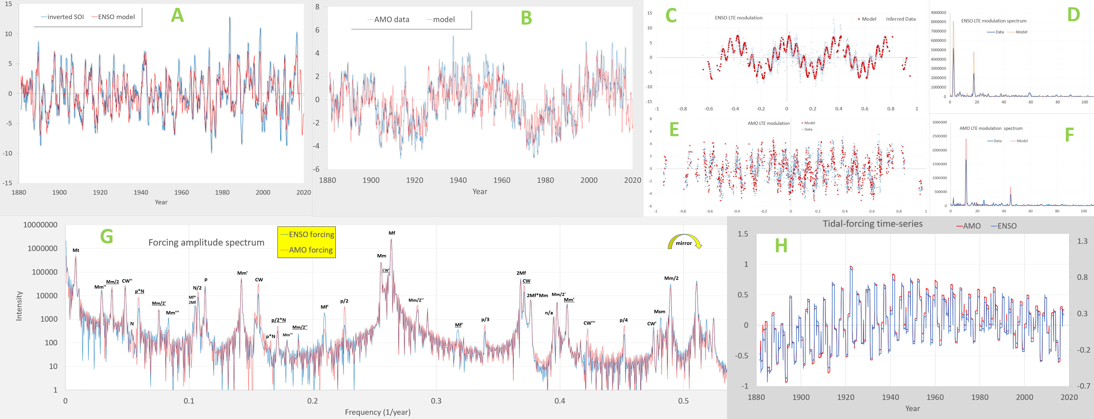
This is the latest product (click to expand)

Read this backwards from H to A.
H = The two tidal forcing inputs for ENSO and AMO — differs really only by scale and a slight offset
G = The constituent tidal forcing spectrum comparison of the two — primarily the expected main constituents of the Mf fortnightly tide and the Mm monthly tide (and the Mt composite of Mf × Mm), amplified by an annual impulse train which creates a repeating Brillouin zone in frequency space.
E&F = The LTE modulation for AMO, essentially comprised of one strong high-wavenumber modulation as shown in F
C&D = The LTE modulation for ENSO, a strong low-wavenumber that follows the El Nino La Nina cycles and then a faster modulation
B = The AMO fitted model modulating H with E
A = The ENSO fitted model modulating the other H with C
Ordinarily, this would take eons worth of machine learning compute time to determine this non-linear mapping, but with knowledge of how to solve Navier-Stokes, it becomes a tractable problem.
Now, with that said, what does this have to do with cross-validation? By fitting only to the ENSO time-series, the model produced does indeed have many degrees of freedom (DOF), based on the number of tidal constituents shown in G. Yet, by constraining the AMO fit to require essentially the same constituent tidal forcing as for ENSO, the number of additional DOF introduced is minimal — note the strong spike value in F.
Since parsimony of a model fit is based on information criteria such as number of DOF, as that is exactly what is used as a metric characterizing order in the previous post, then it would be reasonable to assume that fitting a waveform as complex as B with only the additional information of F cross-validates the underlying common-mode model according to any information criteria metric.
For further guidance, this is an informative article on model selection in regards to complexity — “A Primer for Model Selection: The Decisive Role of Model Complexity“
excerpt:


