
Something I learned early on in my research career is that complicated frequency spectra can be generated from simple repeating structures. Consider the spatial frequency spectra produced as a diffraction pattern produced from a crystal lattice. Below is a reflected electron diffraction pattern of a reconstructed hexagonally reconstructed surface of a silicon (Si) single crystal with a lead (Pb) adlayer ( (a) and (b) are different alignments of the beam direction with respect to the lattice). Suffice to say, there is enough information in the patterns to be able to reverse engineer the structure of the surface as (c).

Now consider the ENSO pattern. At first glance, neither the time-series signal nor the Fourier series power spectra appear to be produced by anything periodically regular. Even so, let’s assume that the underlying pattern is tidally regular, being comprised of the expected fortnightly 13.66 day tropical/synodic cycle and the monthly 27.55 day anomalistic cycle synchronized by an annual impulse. Then the forcing power spectrum of f(t) looks like the RED trace on the left-side of the figure below, F(ω). Clearly that is not enough of a frequency spectra (a few delta spikes) necessary to make up the empirically calculated Fourier series for the ENSO data comprising ~40 intricately placed peaks between 0 and 1 cycles/year in BLUE.

Yet, if we modulate that with an Laplace’s Tidal Equation solution functional g(f(t)) that has a G(ω) as in the yellow inset above — a cyclic modulation of amplitudes where g(x) is described by two distinct sine-waves — then the complete ENSO spectra is fleshed out in BLACK in the figure above. The effective g(x) is shown in the figure below, where a slower modulation is superimposed over a faster modulation.
So essentially what this is suggesting is that a few tidal factors modulated by two sinusoids produces enough spectral detail to easily account for the ~40 peaks in the ENSO power spectra. It can do this because a modulating sinusoid is an efficient harmonics and cross-harmonics generator, as the Taylor’s series of a sinusoid contains an effectively infinite number of power terms.
To see this process in action, consider the following three figures, which features a slider that allows one to get an intuitive feel for how the LTE modulation adds richness via harmonics in the power spectra.
- Start with a mild LTE modulation and start to increase it as in the figure below. A few harmonics begin to emerge as satellites surrounding the forcing harmonics in RED.


2. Next, increase the LTE modulation so that it models the slower sinusoid — more harmonics emerge


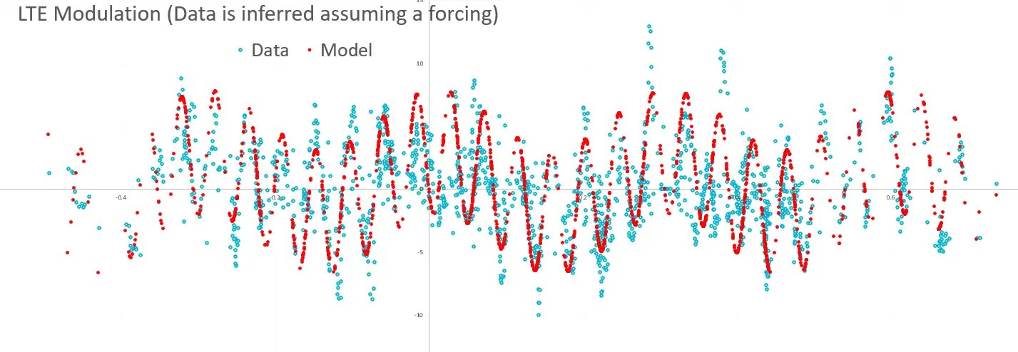
3. Then add the faster sinusoid, to fully populate the empirically observed ENSO spectral peaks (and matching the time series).


It appears as if by magic, but this is the power of non-linear harmonic generation. Note that the peak labeled AB amongst others is derived from the original A and B as complicated satellite-cross terms, which can be accounted for by expanding all of the terms in the Taylor’s series of the sinusoids. This can be done with some difficulty, or left as is when doing the fit via solver software.
To complete the circle, it’s likely that being exposed to mind-blowing Fourier series early on makes Fourier analysis of climate data less intimidating, as one can apply all the tricks-of-the-trade, which, alas, are considered routine in other disciplines.
Individual charts
https://imagizer.imageshack.com/img922/7013/VRro0m.png
https://imagizer.imageshack.com/img924/5325/F6Fn4d.png
https://imagizer.imageshack.com/img923/5339/8ErZMz.png
https://imagizer.imageshack.com/img924/4276/wDNlH0.png
https://imagizer.imageshack.com/img924/8150/bXjihg.png
https://imagizer.imageshack.com/img924/6739/C0aNey.png


