Appendix E of the book contains information on compartmental models, of which resource depletion models, contagion growth models, drug delivery models, and population growth models belong to.
One compartmental population growth model, that specified by the Lotka-Volterra-type predator-prey equations, can be manipulated to match a cyclic wildlife population in a fashion approximating that of observations. The cyclic variation is typically explained as a nonlinear resonance period arising from the competition between the predators and their prey. However, a more realistic model may take into account seasonal and climate variations that control populations directly. The following is a recent paper by wildlife ecologist H. L. Archibald who has long been working on the thesis that seasonal/tidal cycles play a role (one paper that he wrote on the topic dates back to 1977! ).
Our book Mathematical Geoenergy presents a number of novel approaches that each deserve a research paper on their own. Here is the list, ordered roughly by importance (IMHO):
Laplace’s Tidal Equation Analytic Solution. (Ch 11, 12) A solution of a Navier-Stokes variant along the equator. Laplace’s Tidal Equations are a simplified version of Navier-Stokes and the equatorial topology allows an exact closed-form analytic solution. This could classify for the Clay Institute Millenium Prize if the practical implications are considered, but it’s a lower-dimensional solution than a complete 3-D Navier-Stokes formulation requires.
Model of El Nino/Southern Oscillation (ENSO). (Ch 12) A tidally forced model of the equatorial Pacific’s thermocline sloshing (the ENSO dipole) which assumes a strong annual interaction. Not surprisingly this uses the Laplace’s Tidal Equation solution described above, otherwise the tidal pattern connection would have been discovered long ago.
Model of Quasi-Biennial Oscillation (QBO). (Ch 11) A model of the equatorial stratospheric winds which cycle by reversing direction ~28 months. This incorporates the idea of amplified cycling of the sun and moon nodal declination pattern on the atmosphere’s tidal response.
Origin of the Chandler Wobble. (Ch 13) An explanation for the ~433 day cycle of the Earth’s Chandler wobble. Finding this is a fairly obvious consequence of modeling the QBO.
The Oil Shock Model. (Ch 5) A data flow model of oil extraction and production which allows for perturbations. We are seeing this in action with the recession caused by oil supply perturbations due to the Corona Virus pandemic.
The Dispersive Discovery Model. (Ch 4) A probabilistic model of resource discovery which accounts for technological advancement and a finite search volume.
Ornstein-Uhlenbeck Diffusion Model (Ch 6) Applying Ornstein-Uhlenbeck diffusion to describe the decline and asymptotic limiting flow from volumes such as occur in fracked shale oil reservoirs.
The Reservoir Size Dispersive Aggregation Model. (Ch 4) A first-principles model that explains and describes the size distribution of oil reservoirs and fields around the world.
Origin of Tropical Instability Waves (TIW). (Ch 12) As the ENSO model was developed, a higher harmonic component was found which matches TIW
Characterization of Battery Charging and Discharging. (Ch 18) Simplified expressions for modeling Li-ion battery charging and discharging profiles by applying dispersion on the diffusion equation, which reflects the disorder within the ion matrix.
Anomalous Behavior in Dispersive Transport explained. (Ch 18) Photovoltaic (PV) material made from disordered and amorphous semiconductor material shows poor photoresponse characteristics. Solution to simple entropic dispersion relations or the more general Fokker-Planck leads to good agreement with the data over orders of magnitude in current and response times.
Framework for understanding Breakthrough Curves and Solute Transport in Porous Materials. (Ch 20) The same disordered Fokker-Planck construction explains the dispersive transport of solute in groundwater or liquids flowing in porous materials.
Wind Energy Analysis. (Ch 11) Universality of wind energy probability distribution by applying maximum entropy to the mean energy observed. Data from Canada and Germany. Found a universal BesselK distribution which improves on the conventional Rayleigh distribution.
Terrain Slope Distribution Analysis. (Ch 16) Explanation and derivation of the topographic slope distribution across the USA. This uses mean energy and maximum entropy principle.
Thermal Entropic Dispersion Analysis. (Ch 14) Solving the Fokker-Planck equation or Fourier’s Law for thermal diffusion in a disordered environment. A subtle effect but the result is a simplified expression not involving complex errf transcendental functions. Useful in ocean heat content (OHC) studies.
The Maximum Entropy Principle and the Entropic Dispersion Framework. (Ch 10) The generalized math framework applied to many models of disorder, natural or man-made. Explains the origin of the entroplet.
Solving the Reserve Growth “enigma”. (Ch 6) An application of dispersive discovery on a localized level which models the hyperbolic reserve growth characteristics observed.
Shocklets. (Ch 7) A kernel approach to characterizing production from individual oil fields.
Reserve Growth, Creaming Curve, and Size Distribution Linearization. (Ch 6) An obvious linearization of this family of curves, related to Hubbert Linearization but more useful since it stems from first principles.
The Hubbert Peak Logistic Curve explained. (Ch 7) The Logistic curve is trivially explained by dispersive discovery with exponential technology advancement.
Laplace Transform Analysis of Dispersive Discovery. (Ch 7) Dispersion curves are solved by looking up the Laplace transform of the spatial uncertainty profile.
Gompertz Decline Model. (Ch 7) Exponentially increasing extraction rates lead to steep production decline.
The Dynamics of Atmospheric CO2 buildup and Extrapolation. (Ch 9) Convolving a fat-tailed CO2 residence time impulse response function with a fossil-fuel emissions stimulus. This shows the long latency of CO2 buildup very straightforwardly.
Reliability Analysis and Understanding the “Bathtub Curve”. (Ch 19) Using a dispersion in failure rates to generate the characteristic bathtub curves of failure occurrences in parts and components.
The Overshoot Point (TOP) and the Oil Production Plateau. (Ch 8) How increases in extraction rate can maintain production levels.
Lake Size Distribution. (Ch 15) Analogous to explaining reservoir size distribution, uses similar arguments to derive the distribution of freshwater lake sizes. This provides a good feel for how often super-giant reservoirs and Great Lakes occur (by comparison).
The Quandary of Infinite Reserves due to Fat-Tail Statistics. (Ch 9) Demonstrated that even infinite reserves can lead to limited resource production in the face of maximum extraction constraints.
Oil Recovery Factor Model. (Ch 6) A model of oil recovery which takes into account reservoir size.
Network Transit Time Statistics. (Ch 21) Dispersion in TCP/IP transport rates leads to the measured fat-tails in round-trip time statistics on loaded networks.
Particle and Crystal Growth Statistics. (Ch 20) Detailed model of ice crystal size distribution in high-altitude cirrus clouds.
Rainfall Amount Dispersion. (Ch 15) Explanation of rainfall variation based on dispersion in rate of cloud build-up along with dispersion in critical size.
Earthquake Magnitude Distribution. (Ch 13) Distribution of earthquake magnitudes based on dispersion of energy buildup and critical threshold.
IceBox Earth Setpoint Calculation. (Ch 17) Simple model for determining the earth’s setpoint temperature extremes — current and low-CO2 icebox earth.
Global Temperature Multiple Linear Regression Model (Ch 17) The global surface temperature records show variability that is largely due to the GHG rise along with fluctuating changes due to ocean dipoles such as ENSO (via the SOI measure and also AAM) and sporadic volcanic eruptions impacting the atmospheric aerosol concentrations.
GPS Acquisition Time Analysis. (Ch 21) Engineering analysis of GPS cold-start acquisition times. Using Maximum Entropy in EMI clutter statistics.
1/f NoiseModel (Ch 21) Deriving a random noise spectrum from maximum entropy statistics.
Stochastic Aquatic Waves (Ch 12) Maximum Entropy Analysis of wave height distribution of surface gravity waves.
The Stochastic Model of Popcorn Popping. (Appx C) The novel explanation of why popcorn popping follows the same bell-shaped curve of the Hubbert Peak in oil production. Can use this to model epidemics, etc.
Dispersion Analysis of Human Transportation Statistics. (Appx C) Alternate take on the empirical distribution of travel times between geographical points. This uses a maximum entropy approximation to the mean speed and mean distance across all the data points.
Our book Mathematical Geoenergy presents a number of novel approaches that each deserve a research paper on their own (**). Here is the list, ordered roughly by importance (IMHO):
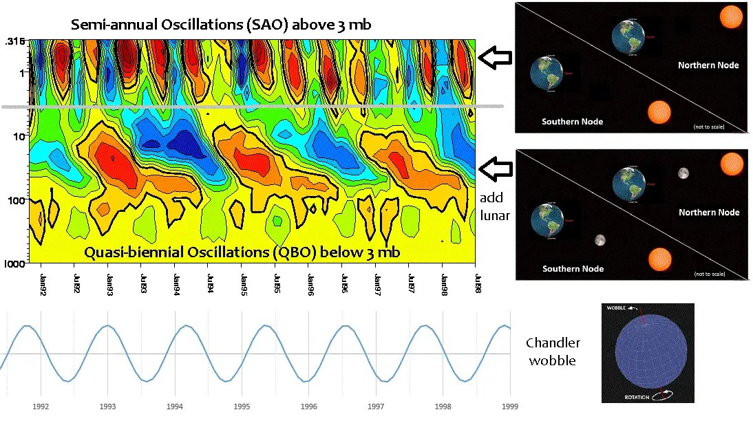
Chapter 11 of the book describes a model for the QBO of stratospheric equatorial winds. The stratified layers of the atmosphere reveal different dependencies on the external forcing depending on the altitude, see Fig 1.
Figure 1 : At high altitudes, only the sun’s annual cycle impacts the stratospheric as a semi-annual oscillation (SAO). Below that the addition of the lunar nodal cycle forces the QBO. The earth itself shows a clear wobble with the lunar cycle interacting with the annual.
Well above these layers are the mesosphere, thermosphere, and ionosphere. These are studied mainly in terms of space physics instead of climate but they do show tidal interactions with behaviors such as the equatorial electrojet [1].
The behaviors known as stratospheric sudden warmings (SSW) are perhaps a link between the lower atmospheric behaviors of equatorial QBO and/or polar vortex and the much higher atmospheric behavior comprising the electrojet. Papers such as [1,2] indicate that lunar tidal effects are showing up in the SSW and that is enhancing characteristics of the electrojet. See Fig 2.
Figure 2 : During SSW events, a strong modulation of period ~14.5 days emerges, close to the lunar fortnightly period as seen in these spectrograms. Taken from ref [2] and see quote below for more info.
“Wavelet spectra of foEs during two SSW events exhibit noticeable enhanced 14.5‐day modulation, which resembles the lunar semimonthly period. In addition, simultaneous wind measurements by meteor radar also show enhancement of 14.5‐day periodic oscillation after SSW onset.”
Tang et al [2]
So the SSW plays an important role in ionospheric variations, and the lunar tidal effects emerge as the higher atmospheric density of a SSW upwelling becomes more sensitive to lunar tidal forcing. That may be related to how the QBO also shows a dependence on lunar tidal forcing due to its higher density.
The Indian Ocean Dipole (IOD) and the El Nino Southern Oscillation (ENSO) are the primary natural climate variability drivers impacting Australia. Contrast that to AGW as the man-made driver. These two categories of natural and man-made causes form the basis of the bushfire attribution discussion, yet the naturally occurring dipoles are not well understood. Chapter 12 of the book describes a model for ENSO; and even though IOD has similarities to ENSO in terms of its dynamics (a CC of around 0.3) the fractional impact of the two indices is ultimately responsible for whether a temperature extreme will occur in a region such as Australia (not to mention other indices such as MJO and SAM).
 One compartmental population growth model, that specified by the Lotka-Volterra-type predator-prey equations, can be manipulated to match a cyclic wildlife population in a fashion approximating that of observations. The cyclic variation is typically explained as a nonlinear resonance period arising from the competition between the predators and their prey. However, a more realistic model may take into account seasonal and climate variations that control populations directly. The following is a recent paper by wildlife ecologist H. L. Archibald who has long been working on the thesis that seasonal/tidal cycles play a role (one paper that he wrote on the topic dates back to 1977! ).