In Chapter 12 of the book, we presented a math model for the equatorial Pacific ocean dipole known as ENSO (El Nino /Southern Oscillation). We argued that the higher wavenumber (×15 of the fundamental) characteristic of ENSO was related to the behavior known as Tropical Instability Waves (TIW). Taken together, the fundamental and TIW components provide enough detail to model ENSO at the monthly level. However if we drill deeper, especially with respect to the finer granularity SOI measure of ENSO, there are rather obvious cyclic factors in the 30 to 90 day range that can add even further detail. The remarkable aspect is that these appear to be related to the behavior known as the Madden-Julian Oscillation (MJO), identified originally as a 40-50 day oscillation in zonal wind [1].
The key to making an association between SOI and MJO is to analyze the daily measure of SOI and compare that to a high-resolution (pentad=5-day) time-series of MJO. Consider if the MJO traveling wave (see Fig 1) is kicked off by the ENSO equatorial disturbance, then an index such as SOI should lead MJO by ~20 days if MJO is traveling at 5 to 15 m/s and it has to fully propagate to be precisely measured.

Indeed, the SOI leads MJO by ~21 days according to this optimal overlay:
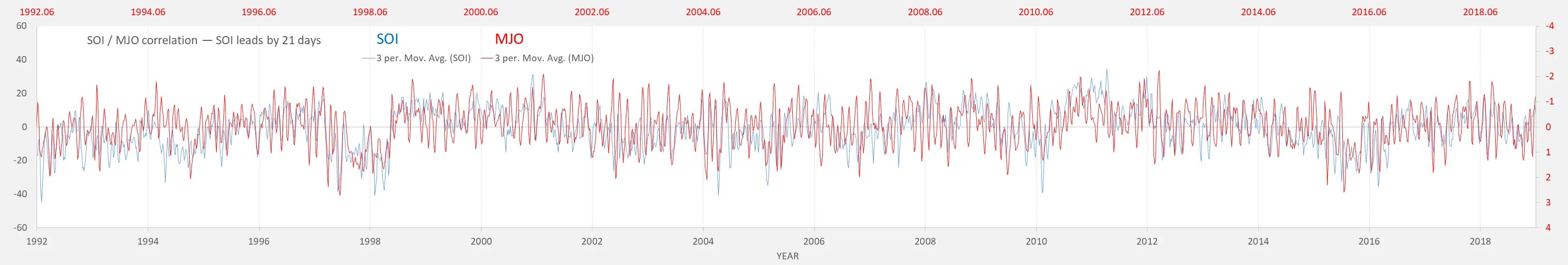
As an aside, one can now see why the high resolution of SOI is necessary. The issue with the monthly SOI readings is that if the MJO period is ~45 days, that’s above the Nyquist frequency, so it would be challenging to isolate these features via sampling the monthly time-series (I have tried and had little success).
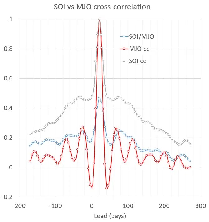
Fig 3 below shows that the correlation is ~0.47 at lead of 21 days and damps quickly with lead/lag shifts of a few days. The 2nd-order satellite wings are at +78 and -25, which would put the MJO period at around 57 to 46 days, which is a sanity check for the MJO typical range.
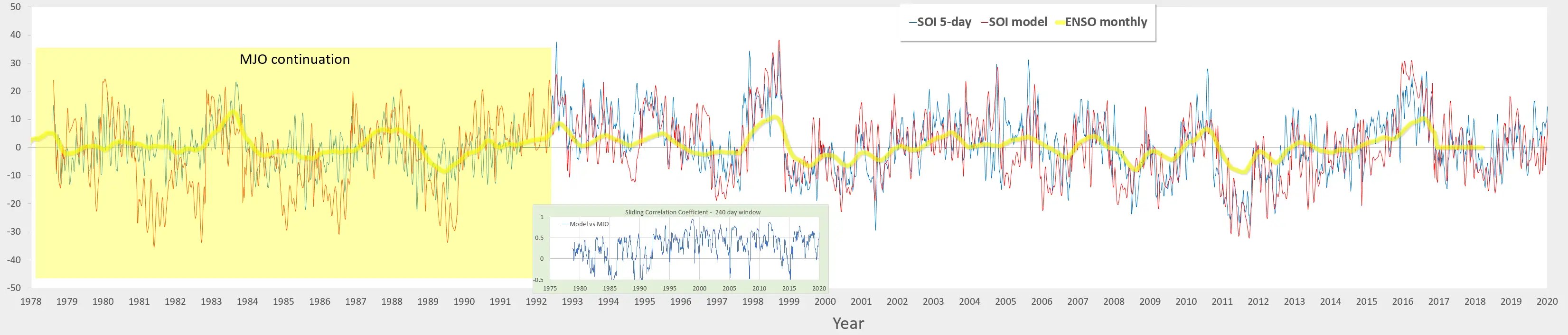
Revisiting the high resolution SOI model, but applying it to the MJO time-series, Fig 4 below shows that a good correlation can be achieved by assuming a nearly identical tidal forcing and similar Laplace Tidal Equation (LTE) modulation parameters.

As a comparison, the high resolution SOI model is shown below. The daily SOI data goes back to 1991, so the MJO data provides the continuation of the time-series prior to that date (but wasn’t applied to the fitting procedure). The parameters and forcing for two models (MJO & SOI) are very similar, yet that should be expected from the known temporal correlation and short lag applied to MJO.
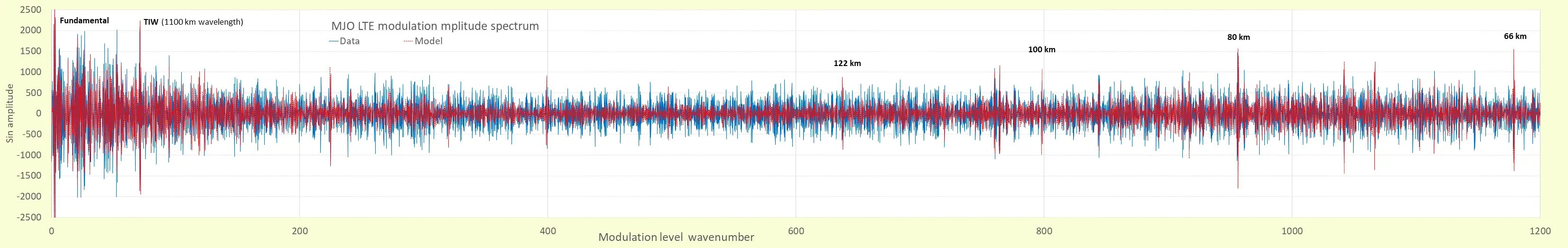
Now comes a novel signal processing algorithm based on the LTE model. We know from the Mach-Zehnder-like modulation of the LTE analytical result that the forcing level replaces the time parameter as the sinusoidal input. So instead of using time for the Fourier spectral analysis, if we use the forcing level then the wavenumber parameters should obviously be revealed in the amplitude spectra. We can then use these directly in the model as a means to quickly tune the fit. This is shown in Fig 6 below for the SOI LTE modulation. The spectra to the left is related to the low frequency aspect of ENSO, while the spikes on the right correspond to the 40 to 50 day MJO cycles.
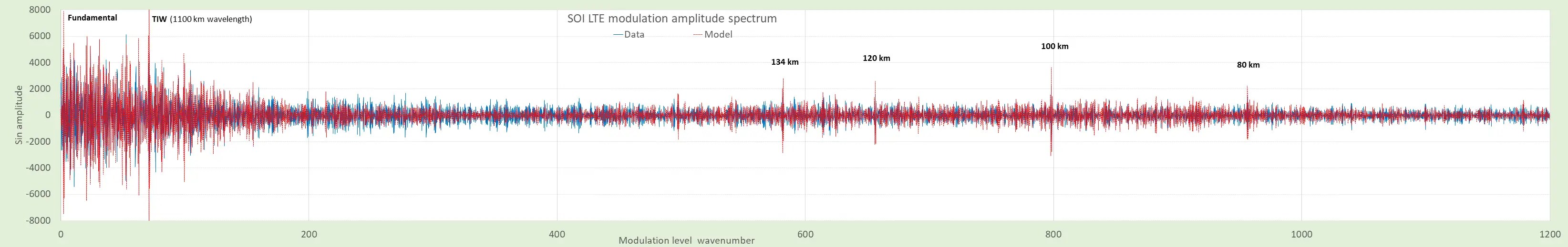
This also applies to the MJO time series with similarly isolated spikes shown in Fig 7. These are sharply delineated wavenumbers that drive the response via the forcing level .
Note that in the the Fourier domain of the actual temporal signal, the addition of a strong single LTE modulation will create a spread response in the spectrum as shown in Fig 8, creating in effect the broad 30 to 90 day spectral spread of MJO. This is just Mach-Zehnder in action, with the temporal => forcing transformation providing a handy adjoint conjugation. So it’s much easier to fit a model to data via Fig. 6 or Fig. 7 than by Fig. 8.

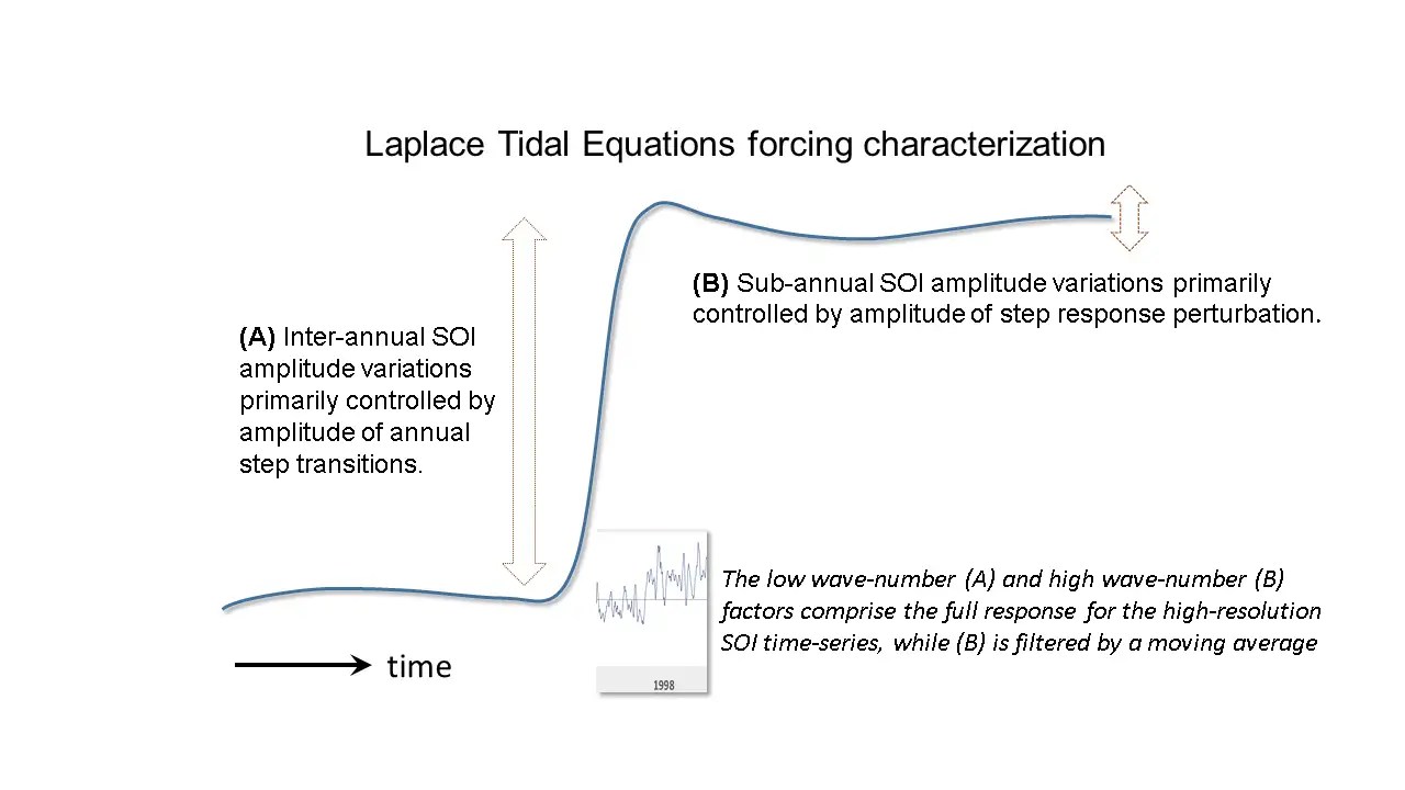
To elaborate further, the reason that these spikes show up so clearly is that they are driven by slight changes in the forcing level, which the Fourier series representation captures by grouping only level shifts, see Fig 9. It thus isolates the standing waves that can develop during the relatively flat tops of the annually-driven step response modulation to tidal forcing. The step change is likely the mechanism that provides a synchronization to the high wavenumber responses and thus long-term coherence between the model and data.
This only explains the math. According to most “just-so” explanations of the MJO behavior [2], a specific location provides the launching pad for the traveling wave to start.
and here’s video I made of a recurring flame soliton running along a groove in a burning oak log. This likely has some of the same math as the MJO, QBO, and Kelvin waves that race around the equator.
References
- Madden R. and P. Julian, 1971: Detection of a 40-50 day oscillation in the zonal wind in the tropical Pacific, J. Atmos. Sci., 28, 702-708.
- Wei, Y., Ren, H.-L., Mu, M. & Fu, J.-X. Nonlinear optimal moisture perturbations as excitation of primary MJO events in a hybrid coupled climate model. Climate Dynamics 54, 675–699 (2020).
Twitter discussion
https://platform.twitter.com/widgets.js
Speaking of solitons, this recent Physical Review Letter cited some of my old work
Hafke, B. et al. Thermally Induced Crossover from 2D to 1D Behavior in an Array of Atomic Wires: Silicon Dangling-Bond Solitons in Si(553)-Au. Physical Review Letters 124, (2020).
https://www.researchgate.net/publication/338522710_Thermally_Induced_Crossover_from_2D_to_1D_Behavior_in_an_Array_of_Atomic_Wires_Silicon_Dangling-Bond_Solitons_in_Si553-Au
This is fascinating in the how the solitons are triggered by increasing thermal energy applied to the step-edge danging bonds. So the “standing waves” of the bonding arrangement release a solition (the equivalent of a traveling wave) which makes it free to slide along the 1D wire.
Perhaps some aspect of topological insulator behavior to this as well.
http://imageshack.com/a/img924/2396/YUzMNx.gif
(Mach-Zehnder type effect — https://www.nature.com/articles/srep14136)
A few thoughts on modeling the SOI and MJO. When I try to fit the MJO and then use that model on the SOI, the fit is surprisingly good in comparison to the SOI fit alone. Even better when I average the SOI and MJO together. The CC on the MJO fit is 0.68 and then when I average in SOI it jumps above 0.7. This indicates that the model is likely trying to find the true value and that true value emerges when the noise is filtered out (which would happen when the two observational time series are averaged).
https://imagizer.imageshack.com/img921/7305/bXNFwm.png
Something to consider is a sliding window CC between MJO and SOI with a window of a few weeks or months and then using that to check on where the model fits the worst. If it’s anything like the NINO34 and SOI, where those two don’t correlate well is where the model fit is worse.
Pingback: Australia Bushfire Causes | GeoEnergy Math
Pingback: EGU 2020 Notes | GeoEnergy Math
They consider the MJO mysterious
https://eos.org/editors-vox/mysterious-engine-of-the-madden-julian-oscillation
https://eos.org/wp-content/uploads/2020/06/2020GL087182-Figure-2-sized-800-wide-1536×1120.jpg
OK, here is substantiation of the analysis above, with the key aspect being the MJO as a traveling wave offshoot of ENSO:
https://platform.twitter.com/widgets.js
Traveling wave offshoot — derived
https://imagizer.imageshack.com/img923/7549/XnI7dH.png
Townsend, R. H. D. “Improved asymptotic expressions for the eigenvalues of Laplace’s tidal equations.” Monthly Notices of the Royal Astronomical Society 497.3 (2020): 2670-2679.
https://arxiv.org/pdf/2006.12596.pdf
Kessler, William S. “Is ENSO a cycle or a series of events?.” Geophysical Research Letters 29, no. 23 (2002): 40-1.
“Although recent El Nino events have seen the occurrence of strong intraseasonal winds apparently associated with the Madden–Julian oscillation (MJO), the usual indices of interannual variability of the MJO are uncorrelated with measures of the ENSO cycle“
joke, always “The eigenvalue problem” — misguided
https://journals.ametsoc.org/view/journals/atsc/78/10/JAS-D-21-0071.1.xml
The MJO on the Equatorial Beta Plane: An Eastward-Propagating Rossby Wave Induced by Meridional Moisture Advection
Pingback: Lunar Torque Controls All | GeoEnergy Math