In Chapter 11 of the book, we present the geophysical recipe for the forcing of the QBO of equatorial stratospheric winds. As explained, the fundamental forcing is supplied by the lunar draconic cycle and impulse modulated by a semi-annual (equatorial) nodal crossing of the sun. It’s clear that the QBO cycle has asymptotically approached a value of 2.368 years, which is explained by its near perfect equivalence to the physically aliased draconic period. Moreover, there is also strong evidence that the modulation/fluctuation of the QBO period from cycle to cycle is due to the regular variation in the lunar inclination, thus impacting the precise timing and shape of the draconic sinusoid. That modulation is described in this post.
As the chapter does not go into the detailed nature of the lunisolar orbit, a good review is available at this NASA page. The salient excerpt describes the lunar draconic month variation:
“The mean interval in the periodic variation of both the draconic month and the orbital inclination is 173.3 days. This is the average time it takes for the Sun to travel from one node to the other. It is also equivalent to the interval between the midpoints of two eclipse seasons. The period is slightly less than half a year because of the retrograde motion of the nodes.”
https://eclipse.gsfc.nasa.gov/SEhelp/moonorbit.html#draconic
In accordance with the NASA chart of lunar orbit inclination variation, we apply precisely that phase of modulation on the draconic sinusoid, only varying the strength of the modulation to fit the QBO signal.

Applying this modulation and optimizing its magnitude by performing an iterative least-squares fit to the QBO will increase the correlation coefficient from ~0.6 for the unmodulated draconic cycle to beyond 0.8. It essentially tracks the locations of the sign reversals much better that the pure draconic cycle while not changing the long-term mean of 2.368 year for the QBO period.

This variation also impacts the model for ENSO, as a similarly modulated draconic signal is applied as a forcing. This is the monthly view of the correlation between the two (the daily view generates a finer detail). The correlation coefficient is ~0.65 which is quite good considering that these time-series are fit independently (and no teleconnection assumed between QBO and ENSO, apart from the common-mode gravitational forcing.

As a post-script: It’s perhaps worthwhile to think of this modulation as an amplified forcing due to it’s signalling the points for the alignment of moon and sun in longitude, a la lunar and solar eclipses as described on the NASA site, “the inclination is always near its maximum value for both solar and lunar eclipses “. Because of this alignment, there is likely to be an amplified tidal forcing.
This is a comparison of the frequency spectrum of the modulated draconic signal for QBO and ENSO, indicating the common positions for the 173.3 day modulation on the left and the 2.368 year fundamental aliased QBO period to the right of that peak. These are aliased positions due to the monthly sampling.
https://imagizer.imageshack.com/img924/7058/1yn9a0.png
This is related
https://twitter.com/WHUT/status/1141017641542402048
and more recent discussion considering these papers is here
https://forum.azimuthproject.org/discussion/comment/21145/#Comment_21145
Pingback: North Atlantic Oscillation | GeoEnergy Math
Pingback: Chandler Wobble according to Na | GeoEnergy Math
Pingback: The MJO | GeoEnergy Math
It’s newsworthy when a climate science paper appears in the prestigious Physical Review Letters. This paper concerns the anomaly observed in the QBO in 2016
I had been mostly analyzing the QBO data for altitudes corresponding to 30hPa, but the data at a lower altitude of 70hPa shows much more fine structure — which the tidal model also shows. The positive peaks (westerlies) show an interesting pattern in how they alternate with even and odd subpeaks, which is what the model does — i.e. the annual impulses create that same pattern when multiplied by the monthly draconic cycles.

(The negative peaks (easterlies) appear not quite as regular, so those excursions are suppressed here)
The other aspect concerns the anomaly of 2016. Based on fitting the tidal model, I think the anomaly instead occurred in 2005 as a slight shift in the annual impulse, and that this shift reverted back in 2016. This is supported by the upper and lower chart. The upper chart shows excellent agreement up to 2005, whereby it needs a slight shift (see lower panel) in the annual impulse to get back in phase.
But this shift disappeared in 2016 (i.e. actually an anomaly reversal). The impulse trains are shown as insets, indicating how subtle this shift needs to be to influence the phase of the model.
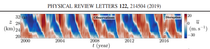
The PRL paper recognizes only the anomaly of 2016, which is obvious to the eye (see below the indicated “disruption”), whereas the anomaly of 2005 is only obvious to the model
What I find disappointing about the full PRL paper is that they can explain an anomaly without truly understanding what causes the QBO. One of the PRL authors is of the same team that published in Science the Topological Origin of Equatorial Waves paper, so they should have done more than just a qualitative study.
Not only this paper but there was another PRL paper on QBO that I missed from last year:
This one is problematic because they create a laboratory experiment that has nothing close to the topological environment of the atmospheric QBO. A rotating upright cylinder with downward gravity is not even close to a spinning sphere with radial gravitational forces and a Coriolis effect
It's newsworthy when a climate science paper appears in the prestigious Physical Review Letters. This paper concerns the anomaly observed in the QBO in 2016>Synopsis:A Missing Beat in Earth’s Oscillating Wind Patterns
>https://physics.aps.org/synopsis-for/10.1103/PhysRevLett.122.214504
I had been mostly analyzing the QBO data for altitudes corresponding to 30hPa, but the data at a lower altitude of 70hPa shows much more fine structure -- which the tidal model also shows. The positive peaks (westerlies) show an interesting pattern in how they alternate with even and odd subpeaks, which is what the model does -- i.e. the annual impulses create that same pattern when multiplied by the monthly draconic cycles.

(The negative peaks (easterlies) appear not quite as regular, so those excursions are suppressed here)
The other aspect concerns the anomaly of 2016. Based on fitting the tidal model, I think the anomaly instead occurred in 2005 as a slight shift in the annual impulse, and that this shift reverted back in 2016. This is supported by the upper and lower chart. The upper chart shows excellent agreement up to 2005, whereby it needs a slight shift (see lower panel) in the annual impulse to get back in phase.
But this shift disappeared in 2016 (i.e. actually an anomaly reversal). The impulse trains are shown as insets, indicating how subtle this shift needs to be to influence the phase of the model.
The PRL paper recognizes only the anomaly of 2016, which is obvious to the eye (see below the indicated "disruption"), whereas the anomaly of 2005 is only obvious to the model
What I find disappointing about the [full PRL paper](https://doi.org/10.1103/PhysRevLett.122.214504) is that they can explain an anomaly without truly understanding what causes the QBO. One of the PRL authors is of the same team that published in Science the [Topological Origin of Equatorial Waves](https://science.sciencemag.org/content/358/6366/1075) paper, so they should have done more than just a qualitative study.
Not only this paper but there was another PRL paper on QBO that I missed from last year:
> "Nonlinear saturation of the large scale flow in a laboratory model of the quasibiennial oscillation"
> https://journals.aps.org/prl/pdf/10.1103/PhysRevLett.121.134502
This one is problematic because they create a laboratory experiment that has nothing close to the topological environment of the atmospheric QBO. A rotating upright cylinder with downward gravity is not even close to a spinning sphere with radial gravitational forces and a Coriolis effect

Pingback: EGU 2020 Notes | GeoEnergy Math
Pingback: Characterizing Wavetrains | GeoEnergy Math
Pingback: Why couldn’t Lindzen figure out QBO? | GeoEnergy Math