Given two models of a physical behavior, the “better” model has the highest correlation (or lowest error) to the data and the lowest number of degrees of freedom (#DOF) in terms of tunable parameters. This ratio CC/#DOF of correlation coefficient over DOF is routinely used in automated symbolic regression algorithms and for scoring of online programming contests. A balance between a good error metric and a low complexity score is often referred to as a Pareto frontier.
So for modeling ENSO, the challenge is to fit the quasi-periodic NINO34 time-series with a minimal number of tunable parameters. For a 140 year fitting interval (1880-1920), a naive Fourier series fit could easily take 50-100 sine waves of varying frequencies, amplitudes, and phase to match a low-pass filtered version of the data (any high-frequency components may take many more). However that is horribly complex model and obviously prone to over-fitting. Obviously we need to apply some physics to reduce the #DOF.
Since we know that ENSO is essentially a model of equatorial fluid dynamics in response to a tidal forcing, all that is needed is the gravitational potential along the equator. The paper by Na [1] has software for computing the orbital dynamics of the moon (i.e. lunar ephemerides) and a 1st-order approximation for tidal potential:

The software contains well over 100 sinusoidal terms (each consisting of amplitude, frequency, and phase) to internally model the lunar orbit precisely. Thus, that many DOF are removed, with a corresponding huge reduction in complexity score for any reasonable fit. So instead of a huge set of factors to manipulate (as with many detailed harmonic tidal analyses), what one is given is a range (r = R) and a declination ( ψ=delta) time-series. These are combined in a manner following the figure from Na shown above, essentially adjusting the amplitudes of R and delta while introducing an additional tangential or tractional projection of delta (sin instead of cos). The latter is important as described in NOAA’s tide producing forces page.

Although I roughly calibrated this earlier [2] via NASA’s HORIZONS ephemerides page (input parameters shown on the right), the Na software allows better flexibility in use. The two calculations essentially give identical outputs and independent verification that the numbers are as expected.
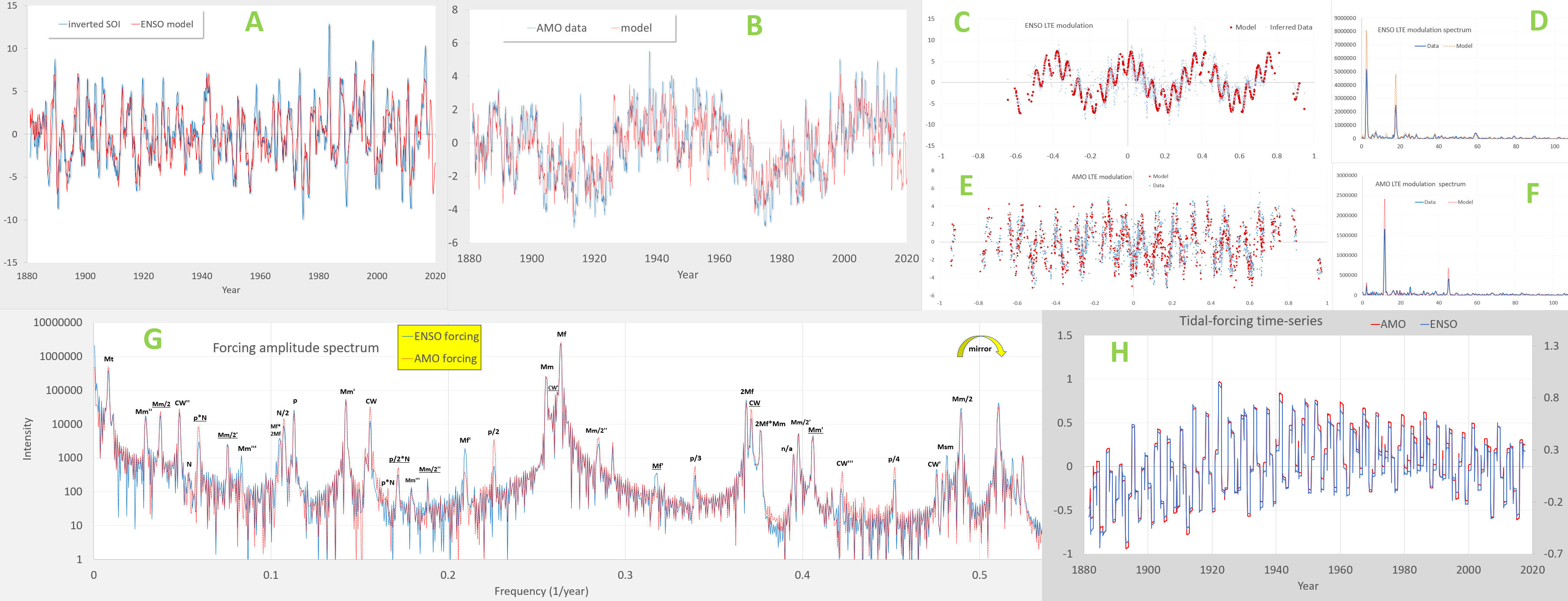
As this post is already getting too long, this is the result of doing a Laplace’s Tidal Equation fit (adding a few more DOF), demonstrating that the limited #DOF prevents over-fitting on a short training interval while cross-validating outside of this band.

or this

This low complexity and high accuracy solution would win ANY competition, including the competition for best seasonal prediction with a measly prize of 15,000 Swiss francs [3]. A good ENSO model is worth billions of $$ given the amount it will save in agricultural planning and its potential for mitigation of human suffering in predicting the timing of climate extremes.
REFERENCES
[1] Na, S.-H. Chapter 19 – Prediction of Earth tide. in Basics of Computational Geophysics (eds. Samui, P., Dixon, B. & Tien Bui, D.) 351–372 (Elsevier, 2021). doi:10.1016/B978-0-12-820513-6.00022-9.
[2] Pukite, P.R. et al “Ephemeris calibration of Laplace’s tidal equation model for ENSO” AGU Fall Meeting, 2018. doi:10.1002/essoar.10500568.1
[3] 1 CHF ~ $1 so 15K = chump change.


