[mathjax]I had this loose thread in the last QBO post:

One caveat in this derivation is that the QBO may actually be the $$v(t)$$ term – the horizontal longitudinal velocity of the fluid, the wind in other words – which can be derived from the above by applying the solution to Laplace’s third tidal equation in simplified form above.

Following up on this gap, I extended the derivation to formally evaluate the velocity.

So from:

and the third simplified Laplace equation

we can derive

So the acceleration of wind, not the velocity, is what obeys the Sturm-Liouville equation. A derivative preserves the periods of the Fourier components, but not the amplitudes, so what we see is a differently shaped envelope for QBO —  i.e. one that is more spiky due to the time derivative applied.

A single lunar Draconic tidal term of $$lambda_d=27.212$$ days multiplied by a yearly modulation sharply peaked at a specific season is enough to capture the QBO acceleration time-series:

The seasonal sharpness is controlled by the power N. This can be approximated as a Fourier series with the same periods found previously: 2.37 years, 0.7 years, 0.41 years, etc.

Fig. 1: The sesonally modulated lunar cycle can be approximated by a sum of Fourier components

This gives the following fit to the QBO acceleration with a correlation coefficient of 0.35 (good, considering the data waveform has no filtering applied and very little optimization went into the fit):

Fig 2:  Modulation of Draconic lunar with seasonal period captures the acceleration of the QBO wind.

The excellent model fit makes sense as the acceleration of wind is simply a F=ma response to a gravitational forcing.

The bottom-line is that this acceleration version of the QBO is much more spiky than the more smoothly oscillating conventional wind speed description of QBO. Yet this spikiness is more closely representative of the seasonally modulated lunar forcing. So what was a caveat in the previous post is now a fundamental revelation which provides an excellent modeling path going forward.

Furthermore, a simple time integration of the acceleration model will recover the wind speed version of the QBO. And fortunately this will retain the same Fourier components that we used earlier to model the QBO, so a self-consistency with the prior model of the QBO is retained.

That’s how a solution should ideally converge — unless one has all the pieces simultaneously, incremental changes to an initial model will provide the process to a solution.

Incidentally, I submitted this research to the AGU meeting for this fall and will find out if the abstract gets accepted in October.

8/28/2016: Additional information pulled from an Azimuth Project forum comment

Deriving the QBO from Laplace’s tidal equations, it becomes apparent that the acceleration of wind and not the wind speed is the fundamental measure to characterize. With that premise, things seem to fall into place much more naturally.

First, multiply the nodal/draconic frequency by a sharply peaked yearly modulation and we get the following as a fit for QBO acceleration:

The fitting region is 1970 to 1982, and the rest is extrapolated. The correlation coefficient is not extremely high but note the amount of fine detail that gets exposed by the model.

To get back the wind speed QBO, the curves are integrated

Again the model fitting is only conducted on the interval from 1970 to 1982. Outside of that interval the model doesn’t track every peak but enough of the fine detail is captured that it’s obvious that the model has predictive power.

The supporting experiment involves running a symbolic regression machine learning trial on this same interval.

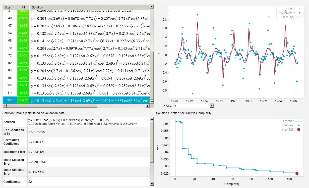
Amazingly, the ML finds all the same harmonics caused by multiplying the sharply peaked yearly signal (freq ~ 2π ) with the Draconic tide (aliased ~2.7 year). No other periods are detected.