Is the equatorial LTE solution a 1-D gyre?

The analytical solution to Laplace’s Tidal Equation along the 1-D equatorial wave guide not only appears odd, but it acts odd, showing a Mach-Zehnder-like modulation which can be quite severe. It essentially boils down to a sinusoidal modulation of a forcing, belonging to a class of non-autonomous functions. The standing wave comes about from deriving a separable spatial component.

sin( f(t) ) sin(kx)

The underlying structure of the solution shouldn’t be surprising, since as with Mach-Zehnder, it’s fundamentally related to a path integral formulation known from mathematical physics. As derived via quantum mechanics (originally by Feynman), one temporally integrates an energy Hamiltonian over a path allowing the wave function to interfere with itself over all possible wavenumber (k) and spatial states (x).

Because of the imaginary value i in the exponential, the result is a sinusoidal modulation of some (potentially complicated) function. Of course, the collective behavior of the ocean is not a quantum mechanical result applied to fluid dynamics, yet the topology of the equatorial waveguide can drive it to appear as one, see the breakthrough paper “Topological Origin of Equatorial Waves” for a rationale. (The curvature of the spherical earth can also provide a sinusoidal basis due to a trigonometric projection of tidal forces, but this is rather weak — not expanding far beyond a first-order expansion in the Taylor’s series)

Moreover, the rather strong interference may have a physical interpretation beyond the derived mathematical interpretation. In the past, I have described the modulation as wave breaking, in that the maximum excursions of the inner function f(t) are folded non-linearly into itself via the limiting sinusoidal wrapper. This is shown in the figure below for progressively increasing modulation.

(click on image to expand)

In the figure above, I added an extra dimension (roughly implying a toroidal waveguide) which allows one to visualize the wave breaking, which otherwise would show as a progressively more rapid up-and-down oscillation in one dimension.

Perhaps coincidentally (or perhaps not) this kind of sinusoidal modulation also occurs in heuristic models of the double-gyre structure that often appears in fluid mechanics. In the excerpt below, note the sin(f(t)) formulation.

The interesting characteristic of the structure lies in the more rapid cyclic variations near the edge of the gyre, which can be seen in an animation (Jupyter notebook code here).

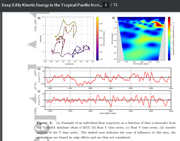
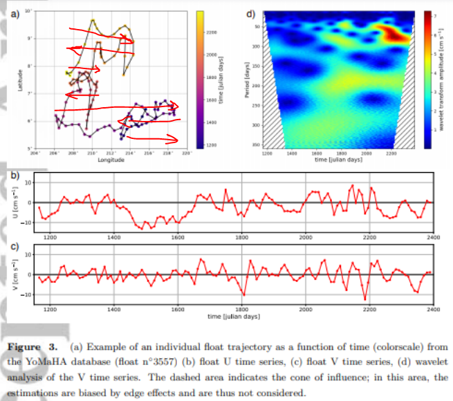
Whether the equivalent of a double-gyre is occurring via the model of the LTE 1-D equatorial waveguide is not clear, but the evidence of double-gyre wavetrains (Lagrangian coherent structures,  Kelvin–Helmholtz instabilities), occurring along the equatorial Pacific is abundantly clear through the appearance of tropical instability (TIW) wavetrains.

These so-called coherent structures may be difficult to isolate for the time being, especially if they involve subtle interfaces such as thermocline boundaries :

“For instance, boundaries of coherent material eddies embracing and transporting volumes of ocean water with different salinity or temperature are notoriously difficult to identify.”

Mercator analysis does show higher levels of waveguide modulation, so perhaps this will be better discriminated over time (see figure below with the long wavelength ENSO dipole superimposed along with the faster TIW wavenumbers in dashed line, with the double-gyre pairing in green + dark purple), and something akin to a 1-D gyre structure will become a valid description of what’s happening along the thermocline. In other words, the wave-breaking modulation due to the LTE modulation is essentially the same as the vortex gyre mapped into a 1-D waveguide.

Reversing Traveling Waves

For the solution to Laplace’s Tidal Equation described in Chapter 12, the spatial and temporal results are separable, leading to a non-linear standing-wave time-series formulation:

sin(kx) sin(A sin(wt) )

By analogy to a linear standing-wave formulation, a solution such as

sin(kx) sin(wt)

with the following traveling wave solution (propagating in the +x direction):

sin(kx-wt)

becomes the following in the non-linear LTE solution mode:

sin(kxA sin(wt) )

This is also a traveling wave, but with the characteristic property of being able to periodically reverse direction from +x to –x depending on the value of A and w. As an intuitive aid, a standing wave can be considered as the superposition of two traveling waves traveling in opposite directions:

sin(kxA sin(wt) ) + sin(kx + A sin(wt) )

Here the cross terms cancel after applying the trig identity on sums, and the separable standing-wave result similar to the first equation results. But, whenever there is an imbalance of +x and -x travelling waves, a periodic reversing traveling-wave/standing-wave mix results. This is shown in the following animation, where a mix of nonlinear traveling-waves and standing-waves show the periodic reversal in direction quite clearly.

This reversal is actually observed in ocean measurements, as exemplified in this recent research article:

From their Figure 3, one can see this reversing process as the trajectory of a measured Argo float drift:

If that is not clear enough, the red arrows in the following annotated figure show the direction of the float motion. The drifting floats may not always exactly follow a trajectory as dictated by the velocity of a traveling wave, as this is partly a phase velocity with limited lateral volume displacement, but clearly a large wave-train such as a Tropical Instability Wave will certainly move a float. At least some of this is due to eddy behavior as the reversal is a natural consequence of a circular vortex motion of a large eddy.

Applying the LTE model to complete spatio-temporal data sets such as what Figure 3 is derived from would likely show an interesting match, adding value to the latest ENSO results, but this will require some digging into the data availability.

Triad Waves

In Chapter 12 of the book, we discuss tropical instability waves (TIW) of the equatorial Pacific as the higher wavenumber (and higher frequency) companion to the lower wavenumber ENSO (El Nino /Southern Oscillation) behavior. Sutherland et al have already published several papers this year that appear to add some valuable insight to the mathematical underpinnings to the fluid-mechanical relationship.

“It is estimated that globally 1 TW of power is transferred from the lunisolar tides to internal tides[1]. The action of the barotropic tide over bottom topography can generate vertically propagating beams near the source. While some fraction of that energy is dissipated in the near field (as observed, for example, near the Hawaiian Ridge [2]), most of the energy becomes manifest as low-mode internal tides in the far field where they may then propagate thousands of kilometers from the source [3]. An outstanding question asks how the energy from these waves ultimately cascades from large to small scale where it may be dissipated, thus closing this branch of the oceanic energy budget. Several possibilities have been explored, including dissipation when the internal tide interacts with rough bottom topography, with the continental slopes and shelves, and with mean flows and eddies (for a recent review, see MacKinnon et al. [4]). It has also been suggested that, away from topography and background flows, internal modes may be dissipated due to nonlinear wave-wave interactions including the case of triadic resonant instability (hereafter TRI), in which a pair of “sibling” waves grow out of the background noise field through resonant interactions with the “parent” wave”

see reference [2]
Continue reading

The MJO

In Chapter 12 of the book, we presented a math model for the equatorial Pacific ocean dipole known as ENSO (El Nino /Southern Oscillation).  We argued that the higher wavenumber (×15 of the fundamental) characteristic of ENSO was related to the behavior known as Tropical Instability Waves (TIW). Taken together, the fundamental and TIW components provide enough detail to model ENSO at the monthly level. However if we drill deeper, especially with respect to the finer granularity SOI measure of ENSO, there are rather obvious cyclic factors in the 30 to 90 day range that can add even further detail. The remarkable aspect is that these appear to be related to the behavior known as the Madden-Julian Oscillation (MJO), identified originally as a 40-50 day oscillation in zonal wind [1].

Continue reading