
click to enlarge
“Nonlinear Differential Equations with External Forcing” presentation starts at slide 2020 http://iclr2020deepdiffeq.rice.edu/ — citation

click to enlarge
“Nonlinear Differential Equations with External Forcing” presentation starts at slide 2020 http://iclr2020deepdiffeq.rice.edu/ — citation
This is a continuation from the previous Length of Day post showing how closely the ENSO forcing aligns to the dLOD forcing.
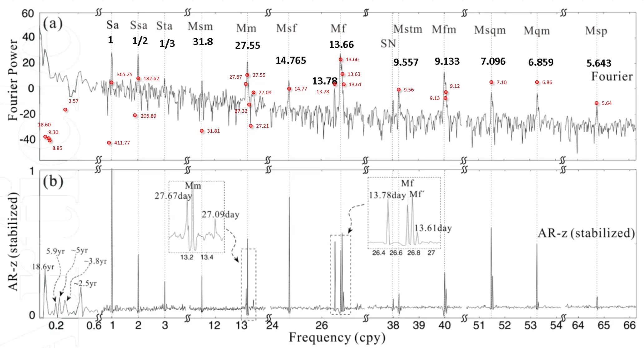
Ding & Chao apply an AR-z technique as a supplement to Fourier and Max Entropy spectral techniques to isolate the tidal factors in dLOD
The red data points are the spectral values used in the ENSO model fit.
The top panel below is the LTE modulated tidal forcing fitted against the ENSO time series. The lower panel below is the tidal forcing model over a short interval overlaid on the dLOD/dt data.

That’s all there is to it — it’s all geophysical fluid dynamics. Essentially the same tidal forcing impacts both the rotating solid earth and the equatorial ocean, but the ocean shows a lagged nonlinear response as described in Chapter 12 of the book. In contrast, the solid earth shows an apparently direct linear inertial response. Bottom line is that if one doesn’t know how to do the proper GFD, one will never be able to fit ENSO to a known forcing.
In Chapter 12 of the book, we discuss tropical instability waves (TIW) of the equatorial Pacific as the higher wavenumber (and higher frequency) companion to the lower wavenumber ENSO (El Nino /Southern Oscillation) behavior. Sutherland et al have already published several papers this year that appear to add some valuable insight to the mathematical underpinnings to the fluid-mechanical relationship.
Continue reading“It is estimated that globally 1 TW of power is transferred from the lunisolar tides to internal tides[1]. The action of the barotropic tide over bottom topography can generate vertically propagating beams near the source. While some fraction of that energy is dissipated in the near field (as observed, for example, near the Hawaiian Ridge [2]), most of the energy becomes manifest as low-mode internal tides in the far field where they may then propagate thousands of kilometers from the source [3]. An outstanding question asks how the energy from these waves ultimately cascades from large to small scale where it may be dissipated, thus closing this branch of the oceanic energy budget. Several possibilities have been explored, including dissipation when the internal tide interacts with rough bottom topography, with the continental slopes and shelves, and with mean flows and eddies (for a recent review, see MacKinnon et al. [4]). It has also been suggested that, away from topography and background flows, internal modes may be dissipated due to nonlinear wave-wave interactions including the case of triadic resonant instability (hereafter TRI), in which a pair of “sibling” waves grow out of the background noise field through resonant interactions with the “parent” wave”
see reference [2]
You really don’t need a supercomputer or petabytes of memory or a high bandwidth network to do climate science.
If you want to learn how to build a climate model, build a climate model. Don’t ask anybody, just build a climate model.

One of the frustrating aspects of climatology as a science is in the cavalier treatment of data that is often shown, and in particular through the potential loss of information through filtering. A group of scientists at NASA JPL (Perigaud et al) and elsewhere have pointed out how constraining it is to remove what are considered errors (or nuisance parameters) in time-series by assuming that they relate to known tidal or seasonal factors and so can be safely filtered out and ignored. The problem is that this is only appropriate IF those factors relate to an independent process and don’t also cause non-linear interactions with the rest of the data. So if a model predicts both a linear component and non-linear component, it’s not helpful to eliminate portions of the data that can help distinguish the two.
As an example, this extends to the pre-mature filtering of annual data. If you dig enough you will find that NINO3.4 data is filtered to remove the annual data, and that the filtering is over-zealous in that it removes all annual harmonics as well. Worse yet, the weighting of these harmonics changes over time, which means that they are removing other parts of the spectrum not related to the annual signal. Found in an “ensostuff” subdirectory on the NOAA.gov site:

Chapter 5 of the book describes a model of the production of oil based on discoveries followed by a sequence of lags relating to decisions made and physical constraints governing the flow of that oil. As it turns out, this so-named Oil Shock Model is mathematically similar to the compartmental models used to model contagion growth in epidemiology, pharmaceutical/drug deliver systems, and other applications as demonstrated in Appendix E of the book.
One aspect of the 2020 pandemic is that everyone with any math acumen is becoming aware of contagion models such as the SIR compartmental model, where S I R stands for Susceptible, Infectious, and Recovered individuals. The Infectious part of the time progression within a population resembles a bell curve that peaks at a particular point indicating maximum contagiousness. The hope is that this either peaks quickly or that it doesn’t peak at too high a level.

