ENSO+QBO Elevator Pitch

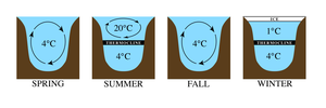
Most papers on climate science take pages and pages of exposition before they try to make any kind of point. The excessive verbiage exists to rationalize their limited understanding of the physics, typically by explaining how complex it all is.

Conversely, think how easy it is to explain sunrise and sunset. From a deterministic point of view [1] and from our understanding of a rotating earth and an illuminating sun, it’s trivial to explain that a sunrise and sunset will happen once each per day. That and perhaps another sentence would be all that would be necessary to write a research paper on the topic …  if it wasn’t already common knowledge. Any padding to this would be unnecessary to the basic understanding. For example, going further and explaining why the earth rotates amounts to answering the wrong question. Thus the topic is essentially an elevator pitch.

If sunset/sunrise is too elementary an example, one could explain ocean tides. This is a bit more advanced because the causal connection is not visible to the eye. Yet all that is needed here is to explain the pull of gravity and the orbital rate of the moon with respect to the earth, and the earth to the sun. A precise correlation between the lunisolar cycles is then applied to verify causality. One could add another paragraph to explain how mixed tidal effects occur, but that should be enough for an expository paper.

We could also be at such a point in our understanding with respect to ENSO and QBO. Most of the past exposition was lengthy because the causal factors could not be easily isolated or were rationalized as random or chaotic. Yet, if we take as a premise that the behavior was governed by the same orbital factors as what governs the ocean tides, we can make quick work of an explanation.
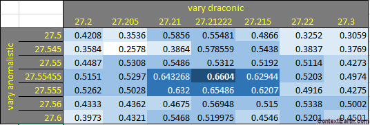
Continue reading

Scaling El Nino

Recently, the rock climber Alex Honnold took a route up El Capitan without ropes.There’s no room to fail at that. I prefer a challenge that one can fail at, and then keep trying.  This is the ascent to conquering El Nino:

The Free-thought Route*

Χ  Base camp:  ENSO (El Nino/Southern Oscillation) is a sloshing behavior, mainly in the thermocline where the effective gravity makes it sensitive to angular momentum changes.
Χ  Faster forcing cycles reinforce against the yearly cycle, creating aliased periods. How?
Χ  Monthly lunar tidal cycles provide the aliased factors: Numbers match up perfectly.
This aliasing also works for QBO, an atmospheric analog of ENSO.
Χ  A biennial meta-stability appears to be active. Cycles reinforce on alternating years.
Χ  The well-known Mathieu modulation used for sloshing simulations also shows a biennial character.
Machine learning experiments help ferret out these patterns.
Χ  The delay differential equation formulation matches up with the biennial Mathieu modulation with a delay of one-year.  That’s the intuitive yearly see-saw that is often suggested to occur.
  The Chandler wobble also shows a tidal forcing tendency, as does clearly the earth’s LOD (length-of-day) variations.
Χ  Integrating the DiffEq model provides a good fit, including long-term coral proxy records
Χ  Solving the Laplace tidal equation via a Sturm-Liouville expression along the equator helps explain details of QBO and ENSO
  Close inspection of sea-level height (SLH) tidal records show evidence of both biennial and ENSO characteristics
Δ Summit: Final validation of the geophysics comparing ENSO forcing against LOD forcing.

Model fits to ENSO using a training interval

The route encountered several dead-ends with no toe-holds or hand-holds along the way (e.g. the slippery biennial phase reversal, the early attempts at applying Mathieu equation). In retrospect many of these excursions were misguided or overly complex, but eventually other observations pointed to the obvious route.

This is a magnification of the fitting contour around the best forcing period values for ENSO. These pair of peak values are each found to be less than a minute apart from the known values of the Draconic cycle (27.2122 days) and Anomalistic cycle (27.5545 days).

The forcing comes directly from the angular momentum variations in the Earth’s rotation. The comparison between what the ENSO model uses and what is measured via monitoring the length-of-day (LOD) is shown below:


*  This is not the precise route I took, but how I wish it was in hindsight.

Strictly Biennial Cycles in ENSO

Continuing from a previous post describing the historical evolution of ocean dynamics and tidal theory, this paper gives an early history of ENSO [1].

The El Niño–Southern Oscillation (ENSO) is among the most pervasive natural climate oscillations on earth, affecting the web of life from plankton to people. During mature El Niño (La Niña) events, the sea surface temperature (SST) in the eastern equatorial Pacific warms (cools), leading to global-scale responses in the terrestrial biosphere transmitted through modifications of large-scale atmospheric circulation. The dynamics of—and global responses to—ENSO have been studied for nearly eight decades (Walker and Bliss 1932; Ropelewski and Halpert 1989; Kiladis and Diaz 1989; Yulaeva and Wallace 1994). Cyclic patterns in climate events have also been connected to something resembling ENSO as early as the mid-nineteenth century. Reminiscing on his 1832 visit to Argentina during his expedition on the H.M.S. Beagle, British naturalist Charles Darwin notes “[t]hese droughts to a certain degree seem to be almost periodical; I was told the dates of several others, and the intervals were about fifteen years” (Darwin 1839). Nearly 60 years later, Darwin enters into his journal “. . . variations in climate sometimes appear to be the effect of the operation of some very general cause” (Darwin 1896). Some believe this “very general cause” was actually an early piecing together of ENSO and its now notorious impact on extreme weather events in South America (Cerveny 2005). It is only a coincidence that Darwin may have been among the first to point out the cyclic nature of ENSO, and the focus of this paper is the association between ENSO and the Galápagos Islands, which also owe their fame to Darwin.

Beyond this history, the purpose of this particular paper is to investigate the mechanics behind ENSO and to isolate the “very general cause” that Darwin first hypothesized (and isn’t it always the case how the most intellectually curious are at the root of scientific investigations?). According to this same paper[1], a “strictly biennial” cycle is routinely observed in ENSO when run with an ocean general circulation model (OGCM). Yet they observe correctly as quoted below that “Such strictly biennial regularity is not realistic, as ENSO in nature at present is neither perfectly regular nor significantly biennial.”

Note how strong the biennial Fourier factor is in their simulation (along with the perfectly acceptable harmonic at 2/3 year which will shape the biennial into anything from a triangle to a square wave). With our ENSO model, I can easily reproduce a strictly biennial cycle just by changing the forcing from a lunar monthly cycle (incongruent with a yearly cycle) to anything that is a harmonic with the yearly cycle. So it’s our claim that it’s the lunar cycle that remains the key factor that changes the ENSO cycle into something that is “neither perfectly regular nor significantly biennial” in the words of the cited paper. The biennial factor is still there but it gets modified and split by the lunar cycle to the extent that no biennial factor remains in the Fourier spectra.

Yet if we look into the GCM’s that researchers have developed and you will find that none have any capabilities for introducing a lunar tidal factor as a forcing.  Why is that?  Probably because someone long ago simply asserted that the lunar gravitational pull wasn’t important for ENSO, contrary to its critical importance for understanding ocean tides.   So is this lunar effect really the “very general cause” that Darwin was thinking of to explain ENSO?

As a result of some intellectual curiosity to actually test the tidal forcing against a biennial modulation, I think the answer is a definitive yes. This is how sensitive the fitting of the model is to selection of the two forcing cycles

By adjusting the values progressively away from the true value for the lunar tidal cycle (27.2122 days for the Draconic cycle and 27.55455 days for the Anomalistic cycle), it will result in a smaller correlation coefficient. This doesn’t happen by accident. Fitting this same model to 200 years of ENSO coral proxy data also doesn’t happen by accident. And extracting precisely phased and correlated lunar cycles to the actual forcing applied to the earth’s rotation also doesn’t happen by accident. I think it’s time for the GCM’s to revisit the role of lunar forcing, just as NASA JPL was about to before they decided to pull the plug on their own lunar research initiative [2].

References

[1] K. B. Karnauskas, R. Murtugudde, and A. J. Busalacchi, “The effect of the Galápagos Islands on ENSO in forced ocean and hybrid coupled models,” Journal of Physical Oceanography, vol. 38, no. 11, pp. 2519–2534, 2008.

[2]  From a post-mortem —  “None of the peer-reviewers nor collaborators in 2006 had anticipated that the most remarkable large-scale process that we were going to find comes from ocean circulations fueled by Luni-Geo-Solar gravitational energy.” 

Overturning Impulse

The only earth science class I took in college was limnology.

Of course I was a casual student of freshwater activities before that time, but certain behaviors of lakes were hammered home by taking this class. For example, the idea behind seasonal lake overturning. The overturning occurs as a singular event at a particular time of the year (monomictic once per year and dimictic twice per year, see figure to the right).

Saltwater doesn’t show the same predilection for overturning as freshwater does, mainly because of the higher density differences above and below the thermocline, but the thermocline does vary, especially at latitudes located off the equator.

The ENSO model that appears so promising might be pointing to a partial overturning  showing a bimictic behavior.  The bi-prefix implies a biennial impulse that reverses direction every year, tied into a biennial Mathieu modulation associated with fluid sloshing dynamics. The Mathieu modulation is partially induced from the forcing conditions [1][2].

The following figure shows the modulation and impulse forcing that generates the best fit for the ENSO model. The BLUE is the Mathieu modulation while the ORANGE is the impulse.

The impulse may be related to a rapidly changing slope when the bimictic partial-overturning kicks in. The positive impulse as the Mathieu modulation moves from high to low, and the negative impulse as the modulation moves from low to high, both occurring at the same relative time late in the year.  Note that the polarity of this may be reversed, as the lunar tidal forcing at the impulse time provides the strength of this forcing through a multiplicative effect. This is shown below.

Whether to call it sloshing or a partial overturning remains to be determined. Yet overall this piece of the puzzle is the primary ansatz behind the entire model — since if we don’t include it, the model does not generate the sharply distinct ENSO peaks and valleys. In other words, this is what causes the physical aliasing necessary to transform the monthly and fortnightly tidal cycles into a more erratic interannual cycling. This is in fact a simple model that shows more complex but still predictable dynamics.

References

[1] T. B. Benjamin and F. Ursell, “The stability of the plane free surface of a liquid in vertical periodic motion,” presented at the Proceedings of the Royal Society of London A: Mathematical, Physical and Engineering Sciences, 1954, vol. 225, pp. 505–515.

[2] S. Bale, K. Clavin, M. Sathe, A. S. Berrouk, F. C. Knopf, and K. Nandakumar, “Mixing in oscillating columns: Experimental and numerical studies,” Chemical Engineering Science, vol. 168, pp. 78–89, 2017.

ENSO forcing – Validation via LOD data

If we don’t have enough evidence that the forcing of ENSO is due to lunisolar cycles, this piece provides another independent validating analysis. What we will show is how well the forcing used in a model fit to an ENSO time series — that when isolated — agrees precisely with the forcing that generates the slight deviations in the earth’s rotational speed, i.e. the earth’s angular momentum. The latter as measured via precise measurements of the earth’s length of day (LOD).  The implication is that the gravitational forcing that causes slight variations in the earth’s rotation speed will also cause the sloshing in the Pacific ocean’s thermocline, leading to the cyclic ENSO behavior.

Continue reading

ENSO and Fourier analysis

Much of tidal analysis has been performed by Fourier analysis, whereby one can straightforwardly deduce the frequency components arising from the various lunar and solar orbital factors. In a perfectly linear world with only two ideal sinusoidal cycles, we would see the Fourier amplitude spectra of Figure 1.

Fig 1: Amplitude spectra for a signal with two sinusoidal Fourier components. To establish the phase, both a real value and imaginary value is plotted.

Continue reading