[mathjax](update here)
Putting the finishing touches on the ENSO model, I decided to derive the Mathieu modulation of the wave equation. It’s actually a rather obvious simplification of Laplace’s Tidal Equations or the Shallow-water Wave Equation applied along the equator. That last assumption is important as the Coriolis forces are known to cancel at the equator (added: perhaps more precisely Isaac Held explains that it vanishes at the equator — it is both zero and a reversal) and so we can use a small angle approximation to reduce the set of equations to a Mathieu or Hill formulation.
To make the job even easier, the three equations that comprise the the Laplace formulation can be formulated initially in terms of the Laplace tidal operator. Per the recent reference [1], the authors separate the temporal component from the standing-wave spatial component(s) and express the operator concisely via implicit time and wavenumber (see Figure 1).

Fig 1: From [1], formulation of the Laplace Tidal Equation
The first step is to use the small angle approximation to $$phi$$

If $$ sigma gg mu $$ while $$sigma$$ not a function of $$mu$$, then the operator can be reduced to:
![F(Theta) = frac{1}{sigma^2} left( frac{d^2Theta}{dmu^2} - left[frac{s}{sigma} + s^2right] Theta right)](https://s0.wp.com/latex.php?latex=F%28Theta%29+%3D+frac%7B1%7D%7Bsigma%5E2%7D+left%28+frac%7Bd%5E2Theta%7D%7Bdmu%5E2%7D+-+left%5Bfrac%7Bs%7D%7Bsigma%7D+%2B+s%5E2right%5D+Theta+right%29&bg=ffffff&fg=444444&s=0&c=20201002)
The next crucial step is to extract the implicit temporal change from $$mu$$ via the chain rule. Even though $$mu$$ is small, changes in $$mu$$ have to be retained to first-order or else the solution would be static along the equator.

added 6-17-2016: In spirit, the above is close, but not a correct expansion.
The actual chain-rule expansion is a bit more complicated and features first-derivative cross-terms.
Will get to that later, not a big deal.
The second term has the dimensions of a reciprocal latitudinal acceleration. If we assume that $$ mu = mu_0 sin(omega t) $$, then
![F(Theta) = - frac{1}{sigma^2} left( frac{d^2Theta}{d t^2} frac{1}{mu_0 omega^2 sin(omega t)} + left[frac{s}{sigma} + s^2right] Theta right)](https://s0.wp.com/latex.php?latex=F%28Theta%29+%3D+-+frac%7B1%7D%7Bsigma%5E2%7D+left%28+frac%7Bd%5E2Theta%7D%7Bd+t%5E2%7D+frac%7B1%7D%7Bmu_0+omega%5E2+sin%28omega+t%29%7D+%2B+left%5Bfrac%7Bs%7D%7Bsigma%7D+%2B+s%5E2right%5D+Theta+right%29&bg=ffffff&fg=444444&s=0&c=20201002)
With that simplification, we reduce the formulation to a temporal second-order differential equation.
![frac{1}{sigma^2} left( frac{d^2Theta}{d t^2} frac{1}{mu_0 omega^2 sin(omega t)} + left[frac{s}{sigma} + s^2right] Theta right) + gamma Theta = f(t)](https://s0.wp.com/latex.php?latex=frac%7B1%7D%7Bsigma%5E2%7D+left%28+frac%7Bd%5E2Theta%7D%7Bd+t%5E2%7D+frac%7B1%7D%7Bmu_0+omega%5E2+sin%28omega+t%29%7D+%2B+left%5Bfrac%7Bs%7D%7Bsigma%7D+%2B+s%5E2right%5D+Theta+right%29+%2B+gamma+Theta+%3D+f%28t%29&bg=ffffff&fg=444444&s=0&c=20201002)
where f(t) is a forcing added to the right-hand side (RHS).
Moving the $$sin(omega t)$$ from the denominator, we recover the Mathieu-like wave equation formulation:
![frac{d^2Theta}{dt^2} + left[frac{s}{sigma} + s^2 + sigma^2 gamma right] Theta mu_0 omega^2 sin(omega t) = sigma^2 mu_0 omega^2 sin(omega t) f(t)](https://s0.wp.com/latex.php?latex=frac%7Bd%5E2Theta%7D%7Bdt%5E2%7D+%2B+left%5Bfrac%7Bs%7D%7Bsigma%7D+%2B+s%5E2+%2B+sigma%5E2+gamma+right%5D+Theta+mu_0+omega%5E2+sin%28omega+t%29+%3D+sigma%5E2+mu_0+omega%5E2+sin%28omega+t%29+f%28t%29&bg=ffffff&fg=444444&s=0&c=20201002)
For now, the primary objective is to verify the sinusoidal behavior in terms of correlating periodicities. Previously, we determined that the f(t) term was composed of seasonally aliased lunar periods, such as the Draconic 27.2 day cycle. (Recently I also found this term buried in the LOD data.)
And the Mathieu modulation likely includes an annual contribution, and, importantly, a strict biennial cycle $$omega=pi$$, which is both observed and implied based on other climatic measures.
The seasonally aliased 27.2 day cycle generates harmonics in ENSO at the same locations as for QBO
1/T = 1/P + n, where P is the tidal period in years, and n is … -3, -2, -1, 0
so for Draconic, 1/T = 365.242/27.2 = 13.43. Stripping off the integer, the value of 0.43 is apparent (and 0.43-1=-0.57) as the strongest low-frequency factor in the power spectrum of Figure 2. Similarly for the fortnightly Draconic (13.6 day), 1/T = 365.242/13.6 = 27.85, and stripping off the integer, one gets 0.85 (and 0.85-1=-0.15). This also corresponds to the Chandler wobble. And with the multiplicative biennial modulation factor adding a +/- 0.5 to each aliased value, the other candidates are 0.85-0.5 = 0.35, 0.43+0.5 = 0.93 (and -0.57+0.5=-0.07, -0.15-0.5=-0.65). All these values are observed as among the strongest low-frequency components in the power spectrum below.
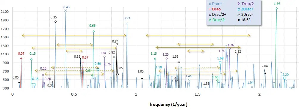
Fig. 2: The strongest components correspond to the seasonally aliased Draconic period. The arrows separate the biennial symmetric terms.
The model fit to the ENSO spectrum is shown in Figure 3. This includes more than the Draconic terms, including potential Tropical fortnight (27.32/2 day) and Anomalistic (27.55 day) terms. Apart from the 1/f filtering envelope, the symmetry about the f=0.5/yr is evident. Note that the power spectrum calculated is essentially the LHS response (data) against the RHS forcing (model). The second derivatives and modulation are included in the LHS, so it is not completely “raw” data.
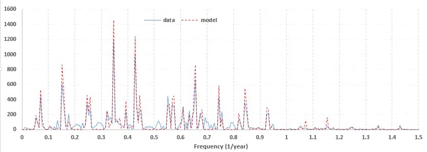
Fig. 3: ENSO power spectrum comparison to model
And in temporal space, the multiple regression fit is shown in Figure 4. Interesting that the correlation coefficient is higher outside the training interval than within the training interval!
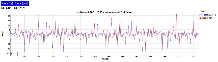
Fig. 4: Fit using the training interval from 1881 to 1950.
This is a very elegant theory in terms of deriving from first-principles; the fact that it is a simplification direct from Pierre Laplace’s original tidal formulation means that we have bypassed sophisticated GCM approaches to potentially solving ENSO . The only caveats to mention are the phase inversion from 1981 to 1996, and the imprecision of the Draconic term, where 27.199 days fits better than 27.212 days. The former aligns with a 7 year interval as there are precisely 94 cycles of 27.199 day periods in 7 years. As ENSO is known to be seasonally aligned, this makes qualitative sense. However, the phase error from that cycle to the actual Draconic cycle will build up over time, and it will eventually go completely out of phase after 70+ years. This actually may be related to the 1981 phase inversion, as that would be a means of re-aligning the phase after a number of years (Another phase inversion may occur prior to 1880, see comment).
The white paper is located on arXiv.
I have to get to work so will leave this post subject to fixing any Latex markup typos later. (Note: fixed some sign-carryover errors due to the 2nd-deriv, same day as posting)
References
[1] Wang, Houjun, John P. Boyd, and Rashid A. Akmaev. “On computation of Hough functions.” Geoscientific Model Development 9.4 (2016): 1477. PDF

BTW, s is the wavenumber and for the primary standing-wave mode of ENSO, it is one of the low-index values, I think 3 is the consensus as that spans the Pacific.
LikeLike
Interesting book Paldor, Nathan. Shallow Water Waves on the Rotating Earth. Springer, 2015.
LikeLike
Pingback: Recent research say QBO frequency is emergent property | context/Earth
Pingback: Ridiculous Paper on Ocean Oscillation | context/Earth
Pingback: Alternate simplification of QBO from Laplace’s Tidal Equations | context/Earth
Pingback: ENSO Model Final Stretch (maybe) | context/Earth
Pingback: Simplifying Laplace’s Tidal Equations for QBO | context/Earth