Climate Dipoles as crystal-crypto

Climate scientists as a general rule don’t understand crystallography deeply (I do). They also don’t understand cryptography (that, I don’t understand deeply either). Yet, as the last post indicated, knowledge of these two scientific domains is essential to decoding dipoles such as the El Nino Southern Oscillation (ENSO). Crystallography is basically an exercise in signal processing where one analyzes electron & x-ray diffraction patterns to be able to decode structure at the atomic level. It’s mathematical and not for people accustomed to existing outside of real space, as diffraction acts to transform the world of 3-D into a reciprocal space where the dimensions are inverted and common intuition fails.

Cryptography in its common use applies a key to enable a user to decode a scrambled data stream according to the instruction pattern embedded within the key. If diffraction-based crystallography required a complex unknown key to decode from reciprocal space, it would seem hopeless, but that’s exactly what we are dealing with when trying to decipher climate dipole time-series -— we don’t know what the decoding key is. If that’s the case, no wonder climate science has never made any progress in modeling ENSO, as it’s an existentially difficult problem.

The breakthrough is in identifying that an analytical solution to Laplace’s tidal equations (LTE) provides a crystallography+cryptography analog in which we can make some headway. The challenge is in identifying the decoding key (an unknown forcing) that would make the reciprocal-space inversion process (required for LTE demodulation) straightforward.

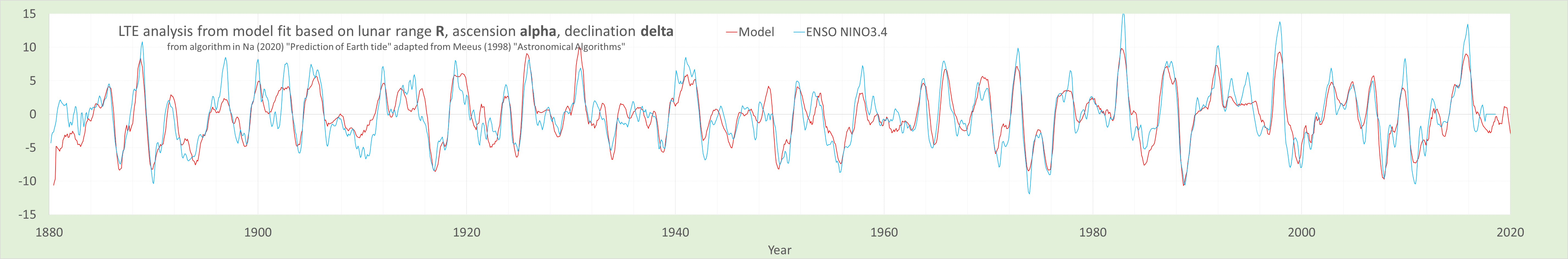
According to the LTE model, the forcing has to be a combination of tidal factors mixed with a seasonal cycle (stages 1 & 2 in the figure above) that would enable the last stage (Fourier series a la diffraction inversion) to be matched to empirical observations of a climate dipole such as ENSO.

The forcing key used in an ENSO model was described in the last post as a predominately Mm-based lunar tidal factorization as shown below, leading to an excellent match to the NINO34 time series after a minimally-complex LTE modulation is applied.

In diffraction terms, the LTE transform from the forcing time series (upper panel)
to the ENSO intensity (lower panel) produces a wave interference relationship

Critics might say and justifiably so, that this is potentially an over-fit to achieve that good a model-to-data correlation. There are too many degrees of freedom (DOF) in a tidal factorization which would allow a spuriously good fit depending on the computational effort applied (see Reference 1 at the end of this post).

Yet, if the forcing key used in the ENSO model was reused as is in fitting an independent climate dipole, such as the AMO, and this same key required little effort in modeling AMO, then the over-fitting criticism is invalidated. What’s left to perform is finding a distinct low-DOF LTE modulation to match the AMO time-series as shown below.

This is an example of a common-mode cross-validation of an LTE model that I originally suggested in an AGU paper from 2018. Invalidating this kind of analysis is exceedingly difficult as it requires one to show that the erratic cycling of AMO can be randomly created by a few DOF. In fact, a few DOFs of sinusoidal factors to reproduce the dozens of AMO peaks and valleys shown is virtually impossible to achieve. I leave it to others to debunk via an independent analysis.

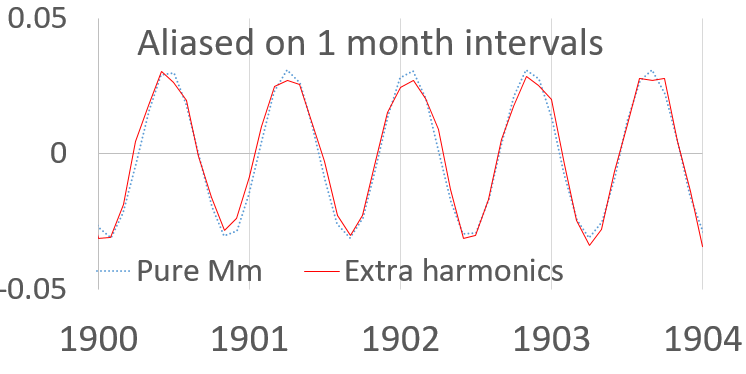
addendum: LTE modulation comparisons, essentially the wavenumber of the diffraction signal:

(click on links to expand)

This is the forcing power spectrum showing the principal Mm tidal factor term at period 3.9 years, with nearly identical spectral profiles for both ENSO and AMO.


According to the precepts of cryptography, decoding becomes straightforward once one knows the key. Similarly, nature often closely guards its secrets, and until the key is known, for example as with DNA, climate scientists will continue to flounder.

References

  1. Chao, B. F., & Chung, C. H. (2019). On Estimating the Cross Correlation and Least Squares Fit of One Data Set to Another With Time Shift. Earth and Space Science, 6, 1409–1415.  https://doi.org/10.1029/2018EA000548
    For example, two time series with predominant linear trends (very low DOF) can have a very high ρ (positive or negative), which can hardly be construed as an evidence for meaningful physical relationship. Similarly, two smooth time series with merely a few undulations of similar timescale (hence low DOF) can easily have a high apparent ρ just by fortuity especially if a time shift is allowed. On the other hand, two very “erratic” or, say, white time series (hence high DOF) can prove to be significantly correlated even though their apparent ρ value is only moderate. The key parameter of relevance here is the DOF: A relatively high ρ for low DOF may be less significant than a relatively low ρ at high DOF and vice versa.


Continue reading

The harmonics generator of the ocean

The research category is topological considerations of Laplace’s Tidal Equations (LTE = a shallow-water simplification of Navier-Stokes) applied to the equatorial thermocline — the following citations provides an evolutionary understanding that I have developed via presentations and publications over the last 6 years (working backwards)

“Nonlinear long-period tidal forcing with application to ENSO, QBO, and Chandler wobble”, EGU General Assembly Conference Abstracts, 2021, EGU21-10515
ui.adsabs.harvard.edu/abs/2021EGUGA..2310515P/abstract

“Nonlinear Differential Equations with External Forcing”, ICLR 2020 Workshop DeepDiffEq 
https://openreview.net/forum?id=XqOseg0L9Q

“Mathematical Geoenergy: Discovery, Depletion, and Renewal”, John Wiley & Sons, 2019, chapter 12: “Wave Energy” 
https://agupubs.onlinelibrary.wiley.com/doi/10.1002/9781119434351.ch12

“Ephemeris calibration of Laplace’s tidal equation model for ENSO”, AGU Fall Meeting 2018, 
https://www.essoar.org/doi/abs/10.1002/essoar.10500568.1

“Biennial-Aligned Lunisolar-Forcing of ENSO: Implications for Simplified Climate Models”,
AGU Fall Meeting 2017, https://www.essoar.org/doi/abs/10.1002/essoar.b1c62a3df907a1fa.b18572c23dc245c9.1

“Analytical Formulation of Equatorial Standing Wave Phenomena: Application to QBO and ENSO”, AGU Fall Meeting Abstracts 2016, OS11B-04, 
ui.adsabs.harvard.edu/abs/2016AGUFMOS11B..04P/abstract

Given that I have worked on this topic persistently over this span of time, I have gained considerable insight into how straightforward it has become to generate relatively decent fits to climate dipoles such as ENSO. Paradoxically, this is both good and bad. It’s good because the model’s recipe is algorithmically simply described in terms of plausibility and parsimony. That’s largely because it’s a straightforward non-linear extension of a conventional tidal analysis model. However that non-linearity opens up the possibility for many similar model fits that are equally good, yet difficult to discriminate between. So it’s bad in the sense that I can come to an impasse in selecting the “best” model.

This is oversimplifying a bit but the framing issue is if you knew the answer was 72, but have a hard time determining whether the question being posed was one of 2×36, 3×24, 4×18, 6×12, 8×9, 9×8, 12×6, 18×4, 24×3, or 36×2. Each gives the right answer, but potentially not the right mechanism. This is a fundamental problem with non-linear analysis.

A conventional tidal analysis by itself is just a few fundamental tidal factors (exactly 4) but made devastatingly accurate by the introduction of 2nd-order harmonics and cross-harmonics. All these harmonics are generated by non-linear effects but the frequency spectrum is so clean and distinct for a sea-level-height (SLH) time-series that the equivalent solution to k × F = 72 is essentially a scaling identification problem where the k is the scale factor for the corresponding cyclic tidal factors F.

Yet, by applying the non-linear LTE solution to the problem of modeling ENSO, we quickly discover that the algorithm is a wickedly effective harmonics and cross-harmonics generator. Any number of combinations of harmonics can develop an adequate fit depending on the variable LTE modulation applied. So it could be a small LTE modulation mixed with a wide assortment of tidal factors (the 2×36 case) or it could be a large LTE modulation mixed with a minimum of tidal factors (the 18×4 case). Or it could be something in between (e.g. the 8×9 case). This is all a result of the sine-of-a-sine non-linearity of the LTE formulation, related to the Mach-Zehnder modulation used in optical cryptography applications. The latter bit is the hint that things may not be unambiguously decoded given the fact that M-Z has been discovered to be nature’s own built-in encryption device.

However, there remains lots of light at the end of this tunnel, as I have also discovered that the tidal factor spread is likely largely governed by a single lunar tidal constituent, the 27.55 day anomalistic Mm cycle interfering with an annual impulse. That’s essentially 2 of the 4 tidal factors, with the other 2 lunar factors providing a 2nd-order correction. For the longest time I had been focused on the 13.66 day tropical Mf cycle as that also lead to a decent fit over the years, specifically since the first beat harmonic of the Mf cycle with the annual impulse is 3.8 years while the Mm cycle is 3.9 years. These two terms are close enough that they only go out-of-phase after ~130 years, which is the extent of the ENSO time-series. Only when you try to simplify a model fit by iterating over the space of factor combinations will you discover the difference between 3.8 and 3.9.

In terms of geophysics, the Mf factor is a tractional tidal forcing operating parallel to the ocean’s surface influenced by the moon’s latitudinal declination, while the Mm factor is a largely perpendicular gravitational forcing influenced by the perigean cycle of the Moon-to-Earth distance. The latter may be the “right mechanism” as each can give close to the “right answer”.

So the gist of the fitting observations is that far fewer harmonic factors are required for a decent Mm-based model than for a Mf-based model. This is slightly at the expense of a stronger LTE modulation, but the parsimony of an Mm-based model can’t be beat, as I will show via the following analysis charts…

This is a good model fit based on a slightly modified Mm-based factorization, with a sample-and-hold placed on a strong annual impulse

The comparison of the modified Mm tidal factorization to the pure Mm is below (the reason the 27.55 day periodicity doesn’t appear is because of the monthly aliasing used in plotting).

The slight pattern on top of pure signal is due to a 6-year beat of the Mm period with the 27.212 day lunar draconic pattern indicating the time between equatorial nodal crossings of the moon. This is the strongest factor of the ascension cycle described in the solar and lunar ephemeris published recently by Sung-Ho Na. As highlighted above by numbered cycles, ~20 occur in the span of 120 years.

Below, an expanded look showing how slight a correction is applied

The integrated forcing after the annual impulse is shown below. The sample-and-hold integration exaggerates low-frequency differences so the distinction between the pure Mm forcing and Mm+harmonics is more apparent. The 6-year periodicity is obscured by longer term variations.

The log-scaled power spectra of the integrated tidal forcing is shown below. Note the overwhelmingly strong peak near the 0.25/year frequency (3.9 year cycle). The rest of the peaks are readily matched to periodicities in the Na ephemerides [1] according to their strength.

The LTE modulation is quite strong for this factorization. As shown below, the forcing levels need to sinusoidally fold several times over to match the observed ENSO behavior. See the recent post Inverting non-autonomous functions for a recipe to aid in iterating for the underlying LTE modulation.

The parsimony of this model can’t be emphasized enough. It’s equivalent to the agreement of a conventional tidal forcing analysis to a SLH time-series in that only a single lunar tidal factor accounts for a majority of the modulation. Only the challenge of finding the correct LTE modulation stands in the way of producing an unambiguously correct model for the underlying ENSO behavioral dynamics.

References

[1] Sung-Ho Na, Chapter 19 – Prediction of Earth tide, Editor(s): Pijush Samui, Barnali Dixon, Dieu Tien Bui, Basics of Computational Geophysics, Elsevier, 2021, Pages 351-372, ISBN 9780128205136,
https://doi.org/10.1016/B978-0-12-820513-6.00022-9. (note: the ephemerides for the Earth-Moon-Sun system matches closely the online NASA JPL ephemerides generator available at https://ssd.jpl.nasa.gov/horizons, but this paper is more useful in that it algorithmically states the contributions of the various tidal factors in the source code supplied. Source code also available at https://github.com/pukpr/GeoEnergyMath/tree/master/src)