The Indian Ocean Dipole (IOD) and the El Nino Southern Oscillation (ENSO) are the primary natural climate variability drivers impacting Australia. Contrast that to AGW as the man-made driver. These two categories of natural and man-made causes form the basis of the bushfire attribution discussion, yet the naturally occurring dipoles are not well understood. Chapter 12 of the book describes a model for ENSO; and even though IOD has similarities to ENSO in terms of its dynamics (a CC of around 0.3) the fractional impact of the two indices is ultimately responsible for whether a temperature extreme will occur in a region such as Australia (not to mention other indices such as MJO and SAM).  

The evidence points to a common tidal forcing for the cyclic behavior for the ocean indices. Even though the tidal forcing is allowed to vary slightly, the time-series inevitably matches the pattern as shown in Fig.1, with a cycle of 3.8 years.

From that forcing f(t), the Laplace’s Tidal Equation (LTE) response is straightforwardly an application of a sin(A f(t)) modulation to the appropriate time-series, as shown in Fig 2 below.

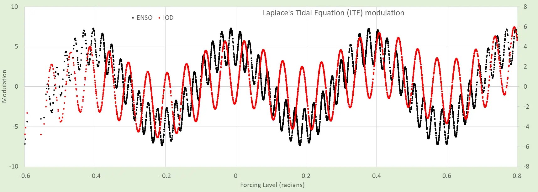
The more gradual wavenumber modulation is the same for each (corresponding to the main ENSO dipole) but the IOD has a much stronger high wavenumber modulation, which is ~ 7× the fundamental.

The best-fit result after applying the appropriate LTE modulation in Fig 2 to Fig 1 is respectively shown in Fig 3 below.

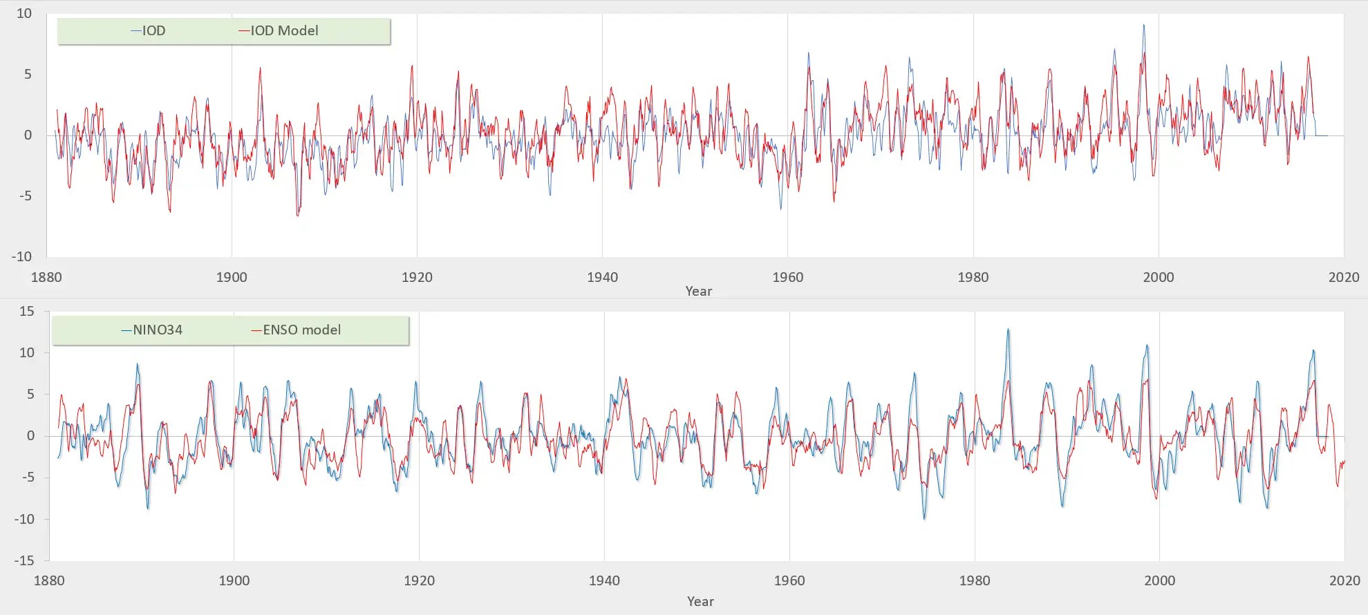
Note what this result is saying : that in each case of a complex erratic cyclic index, a simple modulation can recreate the peaks and valleys remarkably well. This is difficult enough to do for a single index alone but to do it for both simultaneously is statistically impossible given the few degrees of freedom available for such a complex waveform — unless this is the actual standing wave fluid dynamics being modeled.

If this physics model holds up elsewhere, it points to the concept of a universal pattern that we can apply to modeling a standing wave dipole, which is the following data-flow for the LTE model (Fig. 4):

The following paper (thanks to Jim Stuttard @OctupusSnook) provides a way of mathematically thinking about data flows

Paulo Perrone, Notes on Category Theory with examples from basic mathematics (2020)

— from arXiv

In particular, this paper has a very good introduction for scientists and engineers interested in applying category theory to data-flow models. The gist of category theory is to organize mathematical formulations into common canonical patterns such that one can more easily understand what transformations can be applied. It may be coincidental that Perrone chooses just this rarely encountered construction, the LTE modulation highlighted in Fig. 5 below, to introduce the composite data-flow formulation

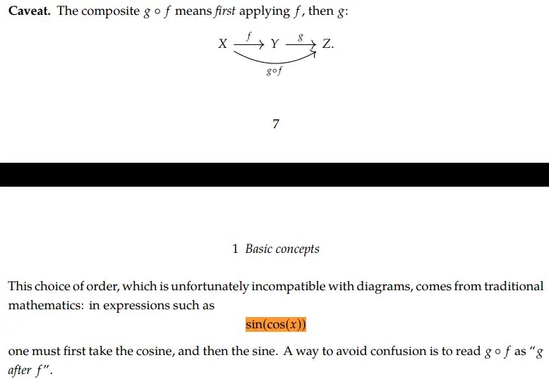
The highlighted text is rare because the units of the inner and outer terms both have to be in radians. This is essentially the same LTE closed-form solution applied to transform Fig 1 and Fig 2 above into Fig 3, with only the sinusoidal LTE modulation differing for ENSO (g1) and IOD (g2) as shown below.

Where else this sin(cos(x)) formulation comes up in is in Mach-Zehnder modulation, where the physical data flow is described by a beam splitter, which mathematically transforms into a composite of a sinusoidally modulated inner phase term.

Follow the development of applied Category Theory at the Azimuth Project forum and we may be able to leverage ideas on how to formulate adjoint and topological transformations — these may be of help in automatically modeling such non-linear constructions.

p.s. Category is an overloaded term as this blog post falls into a Wave Energy category and also a Category Theory category as allowed by WordPress.