In Chapter 11, we developed a general formulation based on Laplace’s Tidal Equations (LTE) to aid in the analysis of standing wave climate models, focusing on the ENSO and QBO behaviors in the book.  As a means of cross-validating this formulation, it makes sense to test the LTE model against other climate indices. So far we have extended this to PDO, AMO, NAO, and IOD, and to complete the set, in this post we will evaluate the northern latitude indices comprised of the Arctic Oscillation/Northern Annular Mode (AO/NAM) and the Pacific North America (PNA) pattern, and the southern latitude index referred to as the Southern Annular Mode (SAM). We will first evaluate AO and PNA in comparison to its close relative NAO and then SAM …

The Pacific North America oscillation stretches across the continent, as described in Wikipedia: “The positive phase of the PNA pattern features above-average barometric pressure heights in the vicinity of Hawaii and over the inter-mountain region of North America, and below-average heights located south of the Aleutian Islands and over the southeastern United States. The PNA pattern is associated with strong fluctuations in the strength and location of the East Asian jet stream.” Both the PNA and the Arctic Oscillation can be easily fit from a perturbation of the NAO model, which can be deduced from the known similarity between the AO and NAO — (“The North Atlantic oscillation (NAO) is a close relative of the AO“).

Fig 1 shows the common tidal forcing for each of these models, with the LTE modulation in the lower panel. The tidal forcing has a strong semi-annual factor, as does the QBO (see Chapter 11).

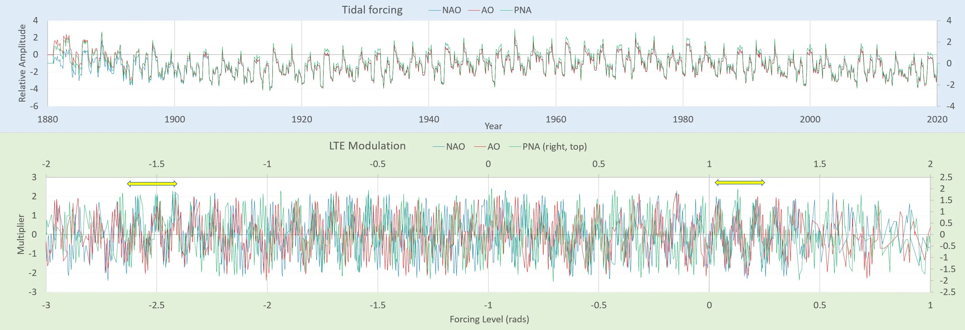
The LTE modulation differs subtly between the three, as the multipliers are slightly different for NAO and AO and within ~15% for PNA. They are in sync at the yellow arrows shown in the lower panel of Fig 1. The LTE modulation is dependent on the fundamental spatial wavenumber defining the dipole, which should be different for each of the regions.

Fig 2 shows the fits for each of the time-series, starting from the NAO described in an earlier post:

You can see how the NAO and AO are vaguely similar and the the PNA is similar but flipped in polarity. It is known that the QBO has a connection to the polar vortex, so the semi-annual commonality between QBO and AO makes some sense [1].

The only major index left is the Southern Annular Mode (SAM) index associated with the Antarctic Oscillation (data source). As a side note and based of the complexity of these waveforms, this should have taken a long time to adequately fit a model if starting from scratch. Yet, since the tidal forcing is nearly identical for each of these indices (see Fig 3 below), the computation took relatively little time to converge to a good fit.

The LTE modulation of SAM was close to that of the complementary AO/NAM, as it retains the same phase over a greater range of forcing levels (indicated by the yellow arrow in Fig 4):

Like the others, the fit for SAM is also very good (Fourier spectrum comparison in lower panel of Fig 5)

As a bottom-line, these climate indices are likely not related as teleconnections (which is the current consensus idea), but more likely by a common-mode forcing . The set is synchronized by the common lunisolar tidal forces operating across the earth and individually distinguished by the standing wave constraints of each region. Moreover, it’s highly unlikely that the quality of these model fits is due to overfitting as there are very few DOF available given the common-mode forcing constraint shared by each model.

In general, what we characterize as the LTE multiplier may require a new vocabulary to describe the resultant behavior. Since there is nothing in the research literature that approximates this solution, there is no lingo or common understanding to draw from. The LTE modulation factor is perhaps something akin to a Reynolds number (Re) or a Richardson number (Ri) defined in fluid dynamics, which makes it a single scalar that describes the breaking or folding of the waves (like a turbulence factor but not chaotic) and relates to the primary wavenumber of the standing wave dipole.

The trend of the LTE value is closer to zero if the climate index is measured close to the equator (QBO is the lowest) and it tends to increase as the index moves away from the equator. The ordering is approximately this:

QBO < ENSO < (AMO ~ IOD) < PDO < ( NAO ~ AO ~ SAM ~ PNA)

The wavenumber of QBO approaches zero because the standing wave encircles the equator and cycles in unison. Correspondingly the wavenumber values may be required to increase away from the equator — where the dimensionality naturally shrinks closer to the poles — but it also may be due to the specific waveguide bounding box of the index. For example, the equatorial Pacific is the widest dimension of the oceanic indices and thus ENSO has the lowest primary wavenumber next to QBO.

The PDO has a significant LTE sin() modulation that is the same as ENSO, but also has a strong factor with a wavenumber that is 5 times as rapid. In contrast the AMO wavenumber modulation is 3 times as fast as ENSO (with a much weaker modulation that’s the same as ENSO). See Fig 6 below.

These also have tidal forcings that are similar (see Fig 7 below) but distinct from that of the upper latitude group of NAO, PNA, AO, and SAM

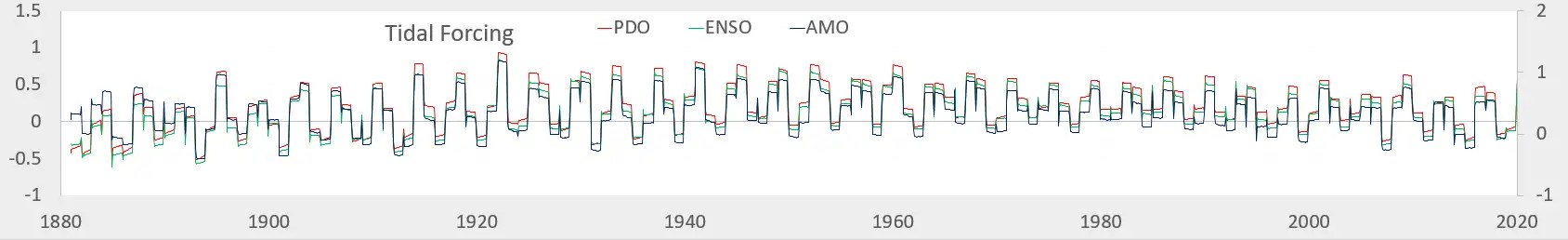
What’s interesting about the common tidal forcing of (AO, NAO, PNA, SAM) is that there is a distinct visible period in the time-series which is the lunar tropical month (27.321582 days) aliased against the annual signal. This can be determined from counting the major periods in Fig 3.

1/(365.242/(27.321582)-13) = 2.72 years

For the QBO, the forcing and response are very close to each other (due to the low LTE factor) and the tidal forcing is the lunar draconic month (27.2122 days) aliased against the annual signal. This gives the measured QBO periodicity of:

1/(365.242/(27.2122)-13) = 2.37 years

There are many papers suggesting that there is a connection between QBO and polar behavior, see [1], but it is not always apparent from the data. The wavenumber=0 symmetry of the QBO precludes any tropical (synodic) dependence so the cycle is draconic while the the other indices require a tropical dependence, as they are geospatially specific. The two distinct cycles will go in and out of sync gradually with an 18.6 year cycle.

In conclusion, the commonality of these 9 indices in terms of a common tidal forcing and distinct LTE modulations provides a convincing cross-validation of the LTE formulation described in our book Mathematical Geoenergy.

References

[1] One such paper from earlier this year claiming a QBO to AO teleconnection:  Observed and Simulated Teleconnections Between the Stratospheric Quasi‐Biennial Oscillation and Northern Hemisphere Winter Atmospheric Circulation