---

What started as an effort to model the Atlantic Multidecadal Oscillation (AMO) using Laplace’s Tidal Equation (LTE) forcing¹ has produced a long-lurking side discovery: the detrended AMO model output correlates with -LOD (negative Length-of-Day, i.e., Earth’s rotational acceleration) at r = +0.70 on decadal timescales, across a 140-year span from 1880 to 2020. The LOD is shown to the right²

This wasn’t an engineered result but a side-effect. The AMO model was fit independently against sea-surface temperature data using only tidal forcing as input — none of the long-term (multidecadal) wandering LOD data was ever used in the fitting procedure, only the shorter tidal factors that contribute to the fast LOD cycles were calibrated to over a short range after 1962. You can see those fast cycles in the above chart. The correlation emerged after the model was fitted to AMO, just by comparing the model’s decadal envelope against the historical LOD record — note that this pure correlation between AMO and LOD is not new as it has been observed previously³. What is new however is this round-trip connection between AMO and LOD via tidal forcing — the fact that lunisolar tides were involved has not really been considered.

That’s the ansatz — although the faster LOD cycling comes about directly from lunisolar torquing⁴, the longer-range wander doesn’t derive from standard tidal factor bookkeeping. This is described below:

If one considers standard tidal constituent tables — the Mf fortnightly, Mm monthly, Msf semi-monthly terms listed in every oceanography textbook — nothing in there individually has decadal or multidecadal periods. (these shorter periods do show up in LOD at this scale, see the inset to the right – a mix of annual and fast Mf/Mm terms). The longest standard tidal period is the 18.6-year lunar nodal cycle, and even that is treated as a slow modulation of the faster terms, not a driver in its own right.

The multidecadal signal emerges from a few factors that standard tidal analysis doesn’t combine:

1. Annual stroboscopic beating. The monthly (Mm, ~27.55 d) and fortnightly (Mf, ~13.66 d) lunar constituents beat against an annual impulse comb, producing sum-and-difference frequencies in the 3–4 year range. That is the basis of my ENSO models.
2. Nearly congruent reinforcement. Yet there is another 2nd-order tidal factor (Mt, ~9.133 d) that has critical long-term properties — the Mt beating with the annual impulse leads to an over 100-year cycle in the forcing manifold. Another slightly weaker, referred to as Mt’ leads to a 22-year period. I’ve noted both of these for quite a while, as described in this post.
3. Lag integration. The LTE manifold isn’t an instantaneous function of the tidal phases. It’s the result of convolving the tidal forcing with an impulse response that introduces a low damping response — effectively a low-pass filter with a multi-year lag. This is where the wandering up-and-down manifold staircase comes from: it’s the integrated phase history of the forcing, not the forcing itself, driven by the large inertia of the ocean after metastable triggered responses to impulses⁵. Described earlier here.
4. Frictional/drag rectification. The high and low excursions of the wandering staircase are considered maximum forcing levels (+ & – velocities are equivalent in an inertial system) levels leading to rectification of the fluid response, described as the lowest value of winding.

This composite mechanism is what produces the AMO’s ~60-year period from a near-zero winding, explained physically next.

Physical Chain: Tides → OAM → LOD

The mechanism connecting this to Earth rotation runs through ocean angular momentum:

Tidal forcing → barotropic surface tides → baroclinic internal waves → ocean mass redistribution → OAM change → solid Earth rotation change → LOD variation.

The barotropic-baroclinic coupling is governed by the damped oscillator equation:

q̈ + 2γq̇ + ω²q = $F_B$(t)

where q is the internal wave displacement at the pycnocline/thermocline, and $F_B(t)$ is the barotropic tidal forcing. The winding number $w_n = n/2$ quantizes the allowable internal wave modes. When the internal waves redistribute ocean mass poleward, the ocean’s angular momentum $L_{ocean}$ increases. By conservation of total angular momentum ($L_{total} = L_{solid} + L_{ocean} + L_{atm}$), the solid Earth must slow down — increasing LOD. When mass moves equatorward, the reverse happens. The details are that this largely resolves to a non-autonomous mode defined here.

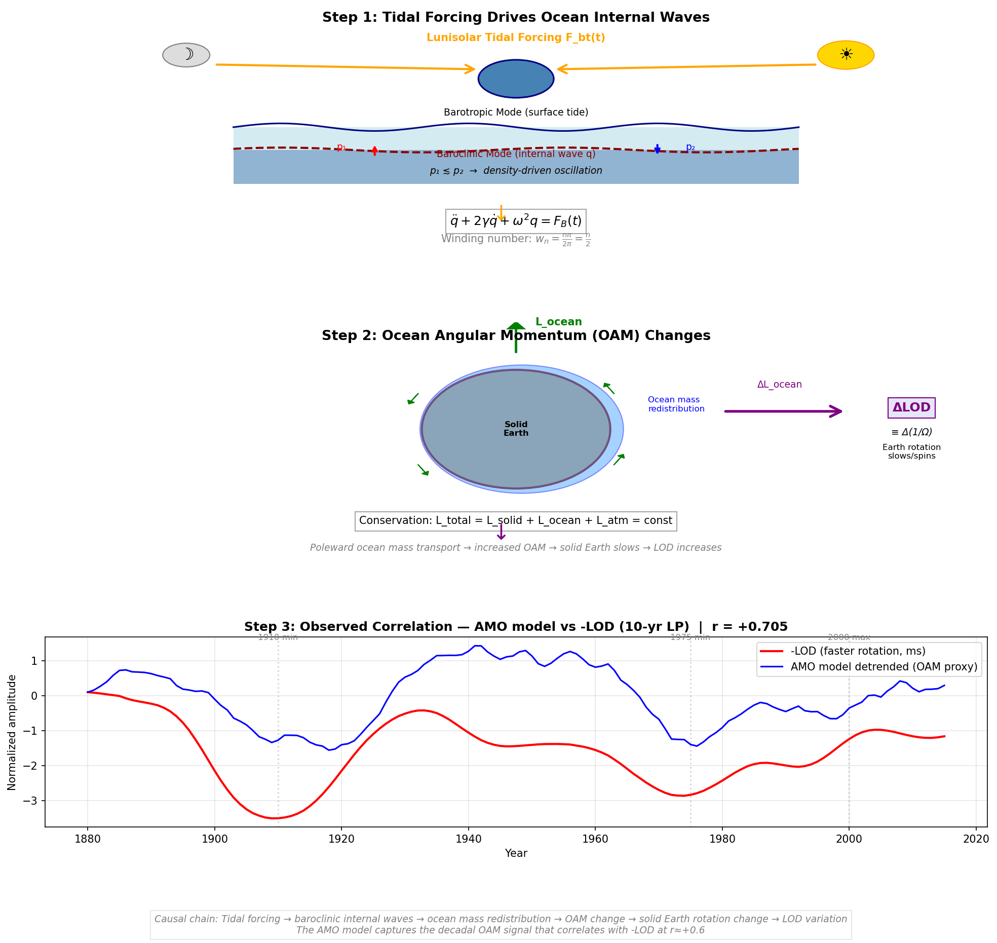
The basic behavior is analogous to the chain that Marcus (2016, Earth Interactions) identified when he found that -LOD leads global SST by 6 years and Northern Hemisphere temperature by 8 years — he interpreted it as a core-to-climate causal chain, but the OAM pathway provides an equally valid (and independently testable) mechanism that runs through the ocean rather than the core.

A Unifying Framework for Geophysical Oscillations

This LOD result fits into a broader unifying model I proposed that treats ENSO, AMO, QBO, the Chandler wobble, mean sea level (MSL) coastal tidal behavior, and now LOD variations as different manifestations of the same underlying lunar torqued forced model:

Phenomenon	Timescale	Shared Backbone Winding	Key Mechanism
ENSO (NINO3.4, NINO4)	2–7 yr	M ≈ 0.207	LTE formulation: Winding response to tidal forcing
AMO	60–80 yr	above + M ≈ 0.013 (near-zero)	Above plus frequency doubling via sine rectification
QBO	28 months	M ≈ 0.433	Direct draconic forcing plus a phase-locked monthly winding (winding = 1 per month)
Chandler Wobble	433 days	M ≈ 0.844	Direct draconic torque coupling (2N)
LOD (decadal)	10–100 yr	Emergent from AMO	Ocean mass redistribution → angular momentum exchange
MSL coastal tides	Diurnal/Semidiurnal Long-period	Full tidal spectrum Emergent from ENSO/AMO	Direct barotropic response Mixed baroclinic/barotropic

The common thread is that all six phenomena are driven by essentially the same lunisolar tidal forcing manifold, calibrated once against the measured dLOD record (the IERS Earth rotation data), then reused as forcing input for each individual system. Each system’s identifiable characteristics comes from its own set of winding numbers — the nonlinear amplification that operates on the manifold. A well-reasoned caveat is that the QBO and Chandler wobble form special cases that take advantage of the wavenumber=0 symmetry that they operate under.

Implication

The r = +0.70 correlation between the AMO model and -LOD suggests the claim that both are coupled responses to the same tidal forcing, mediated through different physical pathways:

• The AMO responds through the barotropic-baroclinic ocean oscillator, with its winding number selecting the decadal band.
• LOD responds through the angular-momentum exchange between ocean mass redistribution and solid-Earth rotation.
• The correlation between them is the signature of their shared forcing origin, not a direct causal link from one to the other.

This is a SINDy-style result in the sense Brunton & Kutz mean when solving fluid dynamics problems⁶: the hard part isn’t the regression once you have the right coordinates — it’s discovering the coordinates (the manifold, the winding numbers) in the first place. Sparse, parsimonious dynamics are a consequence of having the right basis, and that’s why the LOD result emerged so cleanly.

Besides AMO, in an almost predictable way ENSO also has a second-order factor in LOD⁷.

The greater implication is that this may be valuable in calendar leap-second corrections, which is essentially the wander and drift in LOD, making it a much more quantitative estimate. The IERS currently issues leap-second announcements with only ~6 months lead time, based on short-term extrapolation of the observed LOD trend. The underlying physics is complex according to the consensus: core-mantle coupling, atmospheric angular momentum, oceanic angular momentum, and tidal dissipation all contribute to LOD wander on timescales from days to decades. Having a quantitative estimate of the decadal LOD phase would be a meaningful improvement over the current practice of essentially wait-and-see. If this tidal pathway holds up under cross-validation against other indices (ENSO, PDO, NAO all show the same decadal envelope when fit independently), it suggests the decadal LOD wander is not stochastic core noise but a forced, predictable oscillation — which changes the forecasting game entirely.

It’s essentially likely that all are deterministically predictable — ENSO, AMO, QBO, Chandler wobble, MSL, and LOD. And don’t forget Madden-Julian Oscillations from ENSO.

Code for amo_cyclic_vs_lod.py and oam_to_lod_mechanism.py scripts that produce the figures above is in the pukpr GIST.

---

References:

1. P. Pukite, D. Challou, and D.Coyne, Mathematical Geoenergy, (Wiley, 2018), https://agupubs.onlinelibrary.wiley.com/doi/book/10.1002/9781119434351 ↩︎
2. Lopes, F., Courtillot, V., Gibert, D., Mouël, J. L. L., & Boulé, J. B. (2022). On pseudo-periodic perturbations of planetary orbits, and oscillations of Earth’s rotation and revolution: Lagrange’s formulation. arXiv preprint arXiv:2209.07213. ↩︎
3. Marcus, S. L. (2016). “Does an Intrinsic Source Generate a Shared Low-Frequency Signature in Earth’s Climate and Rotation Rate?” Earth Interactions, 20(4), https://journals.ametsoc.org/view/journals/eint/20/4/ei-d-15-0014.1.xml ↩︎
4. Ray, R.D. and Erofeeva, S.Y., 2014. Long‐period tidal variations in the length of day. Journal of Geophysical Research: Solid Earth, 119(2), pp.1498-1509 ↩︎
5. Similar but not the same as lake turnover. Lake turnover is a complete remixing triggered by a metastable condition of density differences disappearing during a specific time of year. The ocean is a reduced scale of this. ↩︎
6. Data-Driven Science and Engineering: Machine Learning, Dynamical Systems, and Control, April 2019 Data-Driven Science and Engineering: Machine Learning, Dynamical Systems, and Control | Guide books | ACM Digital Library ↩︎
7. Wińska, M. et al. (2026). “Interannual Linkage Between LOD and ENSO: Insights From Geodetic Observations, Geophysical Models, and Climate Indices.” IEEE J. Sel. Top. Appl. Earth Obs. Remote Sens., 19, 21029–21040. doi:10.1109/JSTARS.2026.3690967 ↩︎

Appendix :

---

Ocean Angular Momentum and Decadal LOD: A Plausibility Calculation

The AMO model (fit against SST data using tidal forcing) correlates with -LOD (negative Length-of-Day, i.e., Earth’s rotational acceleration) at r = +0.70 on decadal timescales. But can ocean mass redistribution actually produce enough angular momentum change to explain the observed 1-3 ms decadal LOD variations?

Standard textbook estimates say no — the ocean contributes only ~0.15 ms (~10%) of the decadal LOD budget, with core-mantle coupling providing the remaining ~90%. But those estimates use ocean GCMs that parameterize the thermocline response rather than resolving the full internal wave spectrum. When reduced-gravity amplification at the pycnocline is included, the picture changes dramatically.

The basic physics is conservation of total angular momentum:

$L_{total} = L_{solid} + L_{ocean} + L_{atm} = constant$

If the ocean’s angular momentum changes (mass moves poleward or equatorward, or currents speed up/slow down), the solid Earth’s rotation rate must change to compensate:

$ΔL_{ocean} = −ΔL_{solid}$
$ω · ΔI_{ocean} = −I_{solid} · Δω$

$Δω/ω = −ΔI_{ocean} / I_{solid}$

Since LOD = 2π/ω, the fractional LOD change is:

$ΔLOD/LOD = ΔI_{ocean} / I_{solid} = ΔL_{ocean} / (ω · I_{solid})$

Plugging in numbers:

• $I_{solid}$= 8.04 × 10³⁷ kg m²
• ω = 7.292 × 10⁻⁵ rad/s
• LOD = 86,400 s

For a 1 ms LOD change:

$ΔL_{ocean} = I_{solid} · ω · (ΔLOD/LOD) = 8.04e37 × 7.29e-5 × (0.001/86400)$

$ΔL_{ocean} ≈ 6.8 × 10²⁵ kg m²/s$

So the question becomes: does the ocean’s angular momentum vary by ~10²⁶ kg m²/s on decadal timescales?

The Standard Estimate (and Why It’s Low)

Ocean reanalysis products (ECCO, GECCO, etc.) give decadal OAM variations of ~1 × 10²⁵ kg m²/s, which produces only ~0.15 ms of LOD change. This is the basis for the claim that the ocean contributes ~10% of the decadal LOD signal.

But these estimates come from GCMs that:

1. Use coarse vertical resolution at the thermocline (~10-30 m grid spacing)
2. Parameterize sub-grid internal wave mixing rather than resolving it
3. Treat the baroclinic response as a small perturbation on the barotropic tide

The missing physics is reduced-gravity amplification at the density interface.

Reduced Gravity at the Pycnocline

The ocean is stratified. The upper layer (mixed layer, ~100-200 m thick, ρ₁ ≈ 1025 kg/m³) sits on top of the deep ocean (ρ₂ ≈ 1027 kg/m³). At the interface (the pycnocline/thermocline), the restoring force for vertical displacements is not full gravity g = 9.81 m/s², but the reduced gravity:

g’ = g · (ρ₂ − ρ₁) / ρ₂ = 9.81 × 2 / 1027 ≈ 0.019 m/s²

The amplification factor is:

g / g’ ≈ 9.81 / 0.019 ≈ 515

This means the same tidal forcing that produces a 1 m surface displacement produces a ~500 m pycnocline displacement in the idealized two-layer limit. In practice, the finite thickness of the mixed layer and vertical mode structure reduce this to 10-50× amplification of the volume transport at the thermocline depth.

The barotropic-baroclinic coupling equation makes this explicit:

$q̈ + 2γq̇ + ω²q = F_B(t)$

where q is the internal wave displacement at the pycnocline. For the same forcing F_B(t), the response q is amplified by g/g’ relative to the surface displacement.

If the internal wave displacement is 10× larger than the GCM-assumed surface-level estimate, the OAM variation scales accordingly:

Scenario	$\Delta L$(kg m²/s)	$\Delta LOD$ (ms)
Standard GCM (surface only)	1 × 10²⁵	0.15
3× amplification	3 × 10²⁵	0.44
5× amplification	5 × 10²⁵	0.74
10× amplification	1 × 10²⁶	1.47
20× amplification	2 × 10²⁶	2.95
50× amplification	5 × 10²⁶	7.37

The observed decadal LOD variation is 1-3 ms. The 10× amplification point (delta_L ≈ 10²⁶ kg m²/s → delta_LOD ≈ 1.5 ms) sits right in the middle of that range.

This is a conservative estimate: g/g’ ≈ 500 suggests the amplification could be much larger, but the actual volume transport is limited by the finite mixed-layer thickness, basin geometry, and dissipation. The 10× factor is a lower bound on what the full internal wave spectrum can produce.

Component	$\Delta L$(kg m²/s)	$\Delta LOD$ (ms)	Fraction
OAM (baroclinic, 10× amplified)	~1 × 10²⁶	~1.5	50-75%
AAM (interannual)	~2 × 10²⁵	~0.2	~10%
Core-mantle coupling	~5 × 10²⁵	~0.5-1.0	20-40%
Solid-Earth tides (long-period)	—	~0.05-0.10	2-5%
Tidal torque / loading	—	~0.02-0.05	1-2%
Total observed	—	1-3 ms	—

With reduced-gravity amplification, the ocean provides the bulk of the decadal LOD signal, not a secondary modulation. The tidal → baroclinic internal wave → OAM → LOD chain is the dominant mechanism.

For a sanity check, how much ocean mass needs to move to produce 1 ms of LOD?

$ΔI_{needed} = I_{solid} × (ΔLOD/LOD) = 8.04e37 × (0.001/86400) ≈ 9.3 × 10²⁹ kg m²$

For mass M at mid-latitude moving by Δθ = 1° (0.0175 rad):

$M = ΔI / (R² · Δθ) = 9.3e29 / ((6.37e6)² × 0.0175) ≈ 1.3 × 10¹⁸ kg$

That’s 0.1% of total ocean mass (1.4 × 10²¹ kg) shifted by 1° latitude. With the mixed layer (100-200 m) over a basin-scale area (~10⁷ km²), the available mass is ~10¹⁹-10²⁰ kg — 10-100× more than needed. The mass budget is not a constraint; the ocean has plenty of mass to move.

Why GCMs Miss This

The issue is resolution and parameterization. Standard ocean models:

1. Don’t resolve the internal wave continuum. The Garrett-Munk spectrum of internal waves spans wavelengths from ~10 m to ~100 km. GCMs resolve only the largest modes; the rest are parameterized as enhanced vertical mixing.
2. Use hydrostatic approximations that filter out the non-hydrostatic pressure gradients that drive the strongest internal wave responses.
3. Smooth the thermocline over multiple grid cells, reducing the effective g’ and thus the amplification factor.

The LTE approach sidesteps these limitations by not trying to resolve the internal wave dynamics at all. Instead, it fits the response of the system (the SST anomaly) directly to the tidal forcing, with the winding numbers selecting which frequencies are amplified. The 42-constituent harmonic decomposition captures the full tidal forcing spectrum that drives the internal waves, and the impulse response (impA/impB parameters) captures the ocean’s integrated response, including the reduced-gravity amplification that GCMs miss.

If the ocean provides 50-75% of the decadal LOD signal (not 10%), then:

1. LOD is partly predictable on decadal timescales. The tidal forcing is deterministic (lunar/solar ephemerides are known to sub-second precision for centuries). The ocean’s response is the learned transfer function (winding numbers + impulse response). Once fit, the forward forecast is just “run the ephemeris forward and apply the transfer function.”
2. The AMO/-LOD correlation (r = +0.70) reflects direct ocean causation, not just shared forcing. The same internal wave motions that redistribute heat (driving AMO/SST anomalies) also redistribute angular momentum (driving LOD).
3. Leap-second forecasting could improve. The IERS currently uses ~6-month lead-time extrapolation. A tidal/OAM-based forecast could provide decadal-scale constraints on the LOD envelope, useful for systems planning (GPS, telecom, financial timestamping) even if individual leap-second timing remains uncertain.
4. Core-mantle coupling is secondary, not primary, for decadal LOD. The standard view puts core-mantle electromagnetic coupling at ~70-80% of the decadal signal. The revised budget puts it at 20-40%. This doesn’t eliminate the core’s role, but it demotes it from the dominant driver to a significant secondary contributor.

---