This index goes back to 1950. The claim is :

“ As a pattern of internal climate variability, the state of the PNA occasionally changes without a clear and identifiable cause. This reduces the predictability of the PNA and can complicate long-range seasonal weather forecasts. Predictability of the PNA is limited to roughly within 10 days“

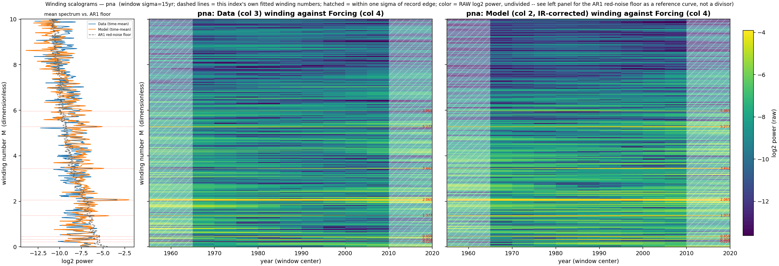
YET, if we apply the universal latent manifold identified via LTE analysis, and invoke a winding scalogram with respect to the data, we find strong continuous ridges indicating a stationary non-autonomous modulation is occurring and is likely causing the PNA cycles. Shown below is the winding scalogram, with the bright yellow indicating integer windings of the fundamental winding at 0.2065, the strongest being $10\times$ of the fundamental (compare this to a strong $6\times$ for the Baltic MSL and SSL)

The physical realization of this is the excellent cross-validated fit using the LTE mapping described in Mathematical Geoenergy, Chapter 12¹ shown below. The region from 1950 to 2001 was used for training, and the region after 2016 was used for predictive tuning, i.e. training produced a multiple regressed set of coefficients that projected into the future based on the manifold. After the training completed, the out-of-band interval shown by the dashed line below was used as a predictive test (the classic train/validate/test CV approach).

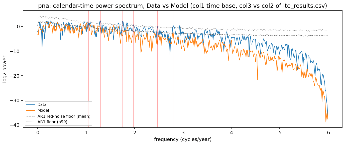
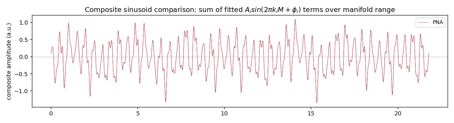
The test interval does show a drop in correlation but that can be expected given the erratic nature of the PNA cycle. This is a cyclic pattern that has eluded climate scientists essentially forever, as it barely exceeds red noise in its power spectrum (right). Yet a handful of winding transformations (with one strong winding, see below) about the manifold, identified by the winding spectrogram, and fitted to the PNA data is able to map the pattern more than good enough to pass a crucial cross-validation test. This is not just predicting past 10 days (as the quote at the top of this post claims), but potentially for years.

How can that be? In other words, how can this have gone unnoticed over decades of analysis? To understand that fully, consider that this LTE formulation falls in the same category as Mach-Zehnder modulation². The complexity of the transfer function in M-Z modulation is of sufficient nonlinearity that it has been used as a practical encryption scheme for analog signals³. The gist of this is that if you don’t know the decryption key, you don’t have a chance of decoding a M-Z encoded signal. But if you do have it, the decryption is concise and fast. There are infinitely many encryption keys possible, so it’s not practical to enumerate and try to discover their value in any systematic way. Applying NVIDIA-powered AI algorithms are of no help here either, as the search space is much too large to explore.

But remember that in our context, nature can narrow down the encryption key possibilities — there aren’t infinitely many to choose from, but instead the ones that make sense are governed by physics and so can be formulated and straightforwardly evaluated. That’s why the LOD-calibrated (from a set of tidal factors) manifold worked — it was essentially the first one that I considered⁴ and have been tweaking for some time, long before the advent of convenient LLM tools. It also makes sense in the case of PNA — the geospatial dynamics of the tri-pole pressure pattern should remind one of amphidromic tidal patterns in the oceans (see right). These are due to the faster conventional diurnal tides, but they hint at how the long-period tidal factors impact the massive inertia of the subsurface waters — as that’s where the source and sink for tropospheric heat resides.

So that explains why this research may succeed — the answer was never really overlooked nor hidden in conventional signal processing artifacts. It was actually uncovered by an educated guess at what the decryption key was. All these ocean indices are falling like dominoes — NINO4, AMO, PDO, any MSL site, etc can be modelled with the LOD-calibrated manifold. Will show the Southern Annular Mode index next go round.

---

Footnotes

1. Pukite P., D. Challou, and D.Coyne, Mathematical Geoenergy, (Wiley, 2018), https://agupubs.onlinelibrary.wiley.com/doi/book/10.1002/9781119434351 ↩︎
2. Pukite, Paul. “Nonlinear Differential Equations with external forcing.” ICLR 2020 Workshop on Integration of Deep Neural Models and Differential Equations. openreview.net/pdf?id=XqOseg0L9Q ↩︎
3. Takiguchi, K. and Ishihara, W., “Encryption of 300 GHz-band wireless signal using optical vector modulator-type encoder”, in Society of Photo-Optical Instrumentation Engineers (SPIE) Conference Series, 2026, vol. 13895, Art. no. 1389506. doi:10.1117/12.3078963;
   Vaidman, L. (1995). “Cryptographic scheme based on a Mach-Zehnder interferometer.” Physical Review Letters, 75(18), 3206. Physical Review Letters. ↩︎
4. Pukite, P.R. “Biennial-Aligned Lunisolar-Forcing of ENSO: Implications for Simplified Climate Models.” AGU Fall Meeting, 2017. https://doi.org/10.1002/essoar.10500568.1 ↩︎