I’m looking at side-band variants of the lunisolar orbital forcing because that’s where the data is empirically taking us. I had originally proposed solving Laplace’s Tidal Equations (LTE) using a novel analytical derivation published several years ago (see Mathematical Geoenergy, Wiley/AG, 2019). The takeaway from the math results — given that LTEs form the primitive basis of the GCM-specific shallow-water approximation to oceanic fluid dynamics — was that my solution involved a specific type of non-linear modulation or amplification of the input tidal. However, this isn’t the typical diurnal/semi-diurnal tidal forcing, but because of the slower inertial response of the ocean volume, the targeted tidal cycles are the longer period monthly and annual. Moreover, as very few climate scientists are proficient at signal processing and all the details of aliasing and side-bands, this is an aspect that has remained hidden (again thank Richard Lindzen for opening the book on tidal influences and then slamming it shut for decades).
Continue readingOcean
Bay of Fundy subbands

With the recent total solar eclipse, it revived lots of thought of Earth’s ecliptic plane. In terms of forcing, having the Moon temporarily in the ecliptic plane and also blocking the sun is not only a rare and (to some people) an exciting event, it’s also an extreme regime wrt to the Earth as the combined reinforcement is maximized.
In fact this is not just any tidal forcing — rather it’s in the class of tidal forcing that has been overlooked over time in preference to the conventional diurnal tides. As many of those that tracked the eclipse as it traced a path from Texas to Nova Scotia, they may have noted that the moon covers lots of ground in a day. But that’s mainly because of the earth’s rotation. To remove that rotation and isolate the mean orbital path is tricky. And that’s the time-span duration where long-period tidal effects and inertial motion can build up and show extremes in sea-level change. Consider the 4.53 year extreme tidal cycle observed at the Bay of Fundy (see Desplanque et al) located in Nova Scotia. This is predicted if the long-period lunar perigee anomaly (27.554 days and the 8.85 absidal precessional return cycle) amplifies the long period lunar ecliptic nodal cycle, as every 9.3 years the lunar path intersects the ecliptic plane, one ascending and the other descending as the moon’s gravitational pull directly aligns with the sun’s. The predicted frequencies are 1/8.85 ± 2/18.6 = 1/4.53 & 1/182, the latter identified by Keeling in 2000. The other oft-mentioned tidal extreme is at 18.6 years, which is identified as the other long period extreme at the Bay of Fundy by Desplanque, and that was also identified by NASA as an extreme nuisance tide via a press release and a spate of “Moon wobble” news articles 3 years ago.
What I find troubling is that I can’t find a scholarly citation where the 4.53 year extreme tidal cycle is explained in this way. It’s only reported as an empirical observation by Desplanque in several articles studying the Bay of Fundy tides.
Continue readingDynamic Time Warping
Useful to note that the majority of the posts written for this blog are in support of the mathematical analysis formulated in Mathematical Geoenergy (Wiley/AGU, 2018). As both new data becomes available and new techniques for model fitting & parameter estimation — aka inverse modeling (predominantly from the machine learning community) — are suggested, an iterative process of validation, fueled by the latest advancements, ensures that the GeoEnergyMath models remain robust and accurately reflective of the underlying observed behaviors. This of course should be done in conjunction with submitting significant findings to the research literature pipeline. However, as publication is pricey, my goal is to make the cross-validation so obvious that I can get an invitation for a review paper — with submission costs waived. Perhaps this post will be the deal-maker — certainly not the deal-breaker, but you can be the judge.
Continue readingFull Wave Forcing
MSet
Global Models of Sea Surface Temperature
These are a set of 6 EOFs that describe the global SST in terms of a set of orthogonal time-series — essentially non-overlapping, each having a cross-correlation of ~0.0 with the others, like a sine/cosine pair, but in both spatial and temporal dimensions.
Continue readingAnnual vs Semi-annual
ENSO models best with alternating sign semi-annual pulses. Operating on the Mf tidal factor this generates a tight forcing with average period 3.8 years.

AMO models best with an annual pulse. Because of the Mt tidal factor the forcing slowly wanders with a period of ~120 years.

PDO models best with an annual pulse but fast decay. Because of the Mt tidal factor the forcing would wander like AMO, but instead it makes biased excursions.

To summarize, the models of ENSO, AMO, and PDO depend on the specific forcing character while keeping the LOD tidal calibration fixed. ENSO likely requires this alternating semi-annual because it is aligned along the equator and so alternates with northern and southern nodal swings. AMO and PDO may require an annual impulse because it’s essentially a northern hemisphere behavior. Why the decay is faster for PDO, or what exactly sets the decay rate after an integrating impulse, is not clear. Perhaps the larger the inertial push the slower the response.
The Power of Darwin
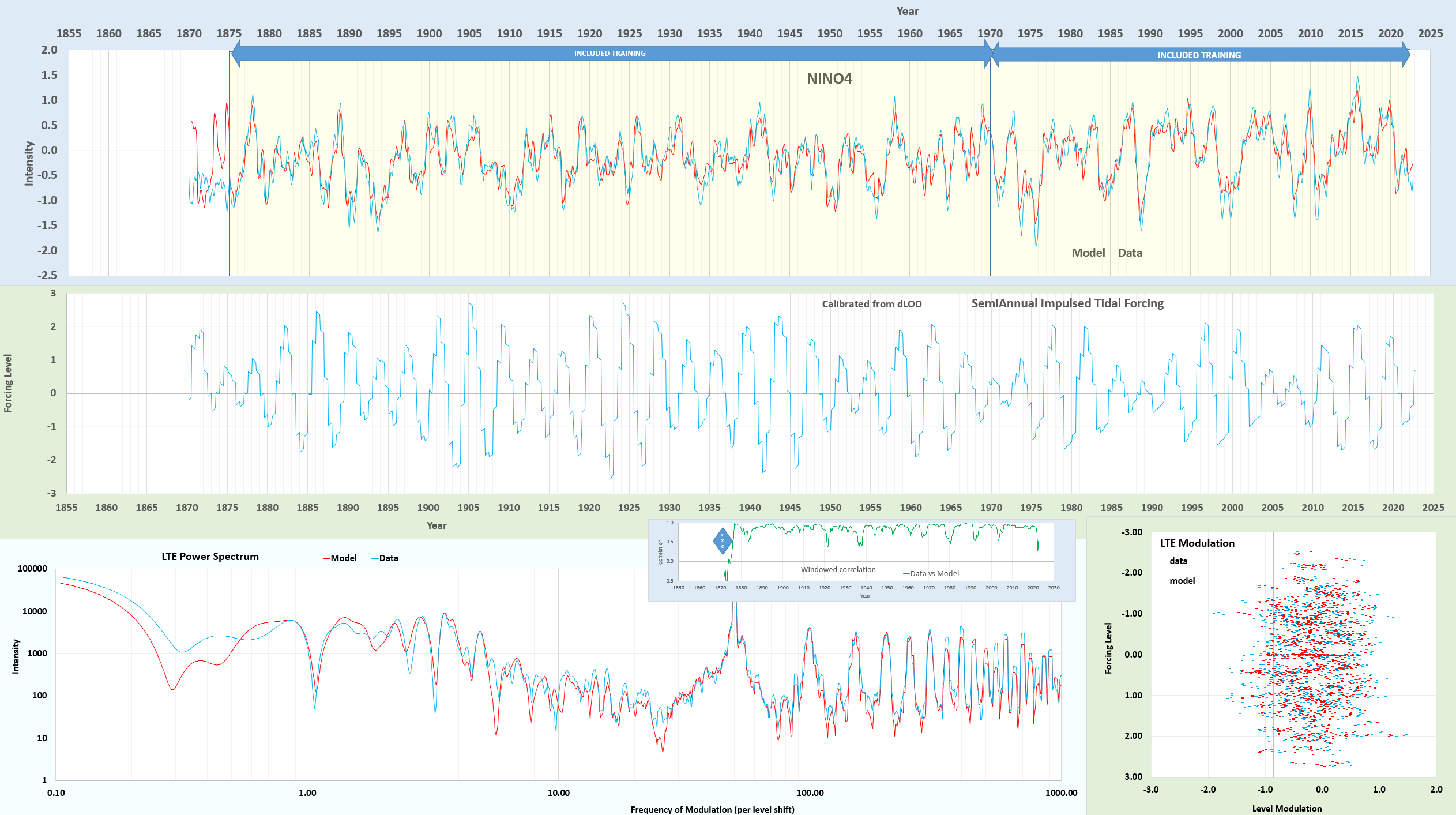
Using the LTE model on the NINO4 ENSO time-series, I excluded the interval between 1870-1875 for cross-validation. The fit below is from scratch on a dLOD-calibrated initial forcing, then allowing the values to vary slightly but the dLOD remains at 0.9999668 of the initial calibration.

The cross-validation doesn’t look good and actually is anti-correlated to a CC = -0.5 over that interval. But the region before 1875 appears suspiciously flat in any case, see the data on the KNMI site — it’s only a certainty that the El Nino peak at 1877-1878 is real and not estimated.
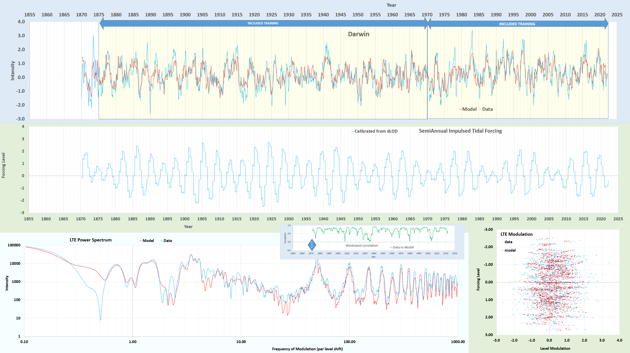
So, the next step is to take the fit to NINO4 and apply it to the Darwin (SOI) time-series, applying the same fitting interval from 1875-present. Immediately, it captures the 3 positive excursions in the interval 1870 to 1875. And then letting the fit proceed to a high CC, the result is shown below:

The resultant fit in the excluded cross-validation region reaches 0.58, thus reversing the anti-correlation and confirming that the NINO4 time-series data prior to 1875 is likely incorrect.
The fit data is at https://gist.github.com/pukpr/c26f1da00337e92dbb47671ca48af2cf?permalink_comment_id=4639783#gistcomment-4639783. The main modifications to tidal factors are in the very long periods — these values start small due to the dLOD calibration (the differential filters out low frequencies) but the 4.42 year amplitude is nearly tripled after the fit, the 8.85 & 9.3 year up by 50%. The 18.6 year is only up 14%, and the 3rd order 6 year and 15.9 year are down 63% and up 45% respectively. All the fortnightly and monthly values are stable. This is perhaps reasonable considering how much the LOD drifts over time at low frequency, and that the calibration is restricted to post-1962.
The Big 10 Climate Indices

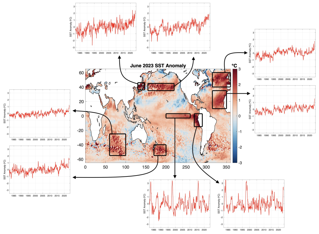
The above diagram courtesy of Karnauskus

Overall I’m confident with the status of the published analysis of Laplace’s Tidal Equations in Mathematical Geoenergy, as I can model each of these climate indices with precisely the same (save one ***) tidal forcing, all calibrated by LOD. The following Threads allow interested people to contribute thoughts
- ENSO – https://www.threads.net/@paulpukite/post/CuWS8MFu8Jc
- AMO – https://www.threads.net/@paulpukite/post/Cuh4krjJTLN
- PDO – https://www.threads.net/@paulpukite/post/Cuu0VCypIi5
- QBO – https://www.threads.net/@paulpukite/post/CuiKQ5tsXCQ
- SOI (Darwin & Tahiti) – https://www.threads.net/@paulpukite/post/Cuu2IkBJh55 => MJO
- IOD (East & West) – https://www.threads.net/@paulpukite/post/Cuu9PYvJAG2
- PNA – https://www.threads.net/@paulpukite/post/CuvAVR7JN7R
- AO – https://www.threads.net/@paulpukite/post/CuvEz37JPFV
- SAM – https://www.threads.net/@paulpukite/post/CuvLZ2CMt1X
- NAO – https://www.threads.net/@paulpukite/post/CuvNnwns2la
(*** The odd-one out is QBO, which is a global longitudinally-invariant behavior, which means that only a couple of tidal factors are important.)
Is the utility of this LTE modeling a groundbreaking achievement? => https://www.threads.net/@paulpukite/post/CuvNnwns2la
Canonical Cross-Validation
The only hope for a non-controlled-experiment-verified model to gain acceptance is either by (1) showing repeated success in predictions, or, precluding that due to long cycle time (2) producing rock-solid cross-validation results. Why? Let ChatGPT-4 answer:
Continue readingWhy is there a tide?
This is the title of Chapter 4 of an Elsevier volume called “Journey through Tides”
| Sophie Ward, David Bowers, Mattias Green, Sophie-Berenice Wilmes, Chapter 4 – Why is there a tide?, Editor(s): Mattias Green, João C. Duarte, A Journey Through Tides, Elsevier, 2023, Pages 81-113, ISBN 9780323908511, https://doi.org/10.1016/B978-0-323-90851-1.00001-7. (https://www.sciencedirect.com/science/article/pii/B9780323908511000017) Abstract: Tides are created by the gravitational pull of the Moon and Sun on the ocean. More exactly, it is the variation in these forces that creates tides. The Earth and Moon are held in orbit by their mutual gravitational attraction. The Moon’s gravity is exactly right at the center of the Earth, but it is a little too strong in the Earth hemisphere facing the Moon and a little too weak in the opposite hemisphere. These discrepancies make the tide generating force. As the Earth spins, the ocean experiences an oscillating force which creates long tide waves – the crest of the wave is the high tide and the trough low tide. In the deep ocean, the amplitude of the tide wave is small, but on the continental shelf, the wave is amplified by resonance, making the large tidal range we see at some coasts. Keywords: Tides; Tide generating force; Cotidal charts; Tidal dynamics; Tidal dissipation |
The domain experts selected to answer this question assert this:
“While this is not an exhaustive list of why the tide is important, it is important to note here that perhaps the most physically far-reaching influence of the tide, long-term, is on the change in day length.”
The day length impact is straight-forward to understand for a rotating solid body as the total angular momentum is conserved between the Earth, smaller Moon, and much larger sun. This is essentially a linear perturbation causing the Earth’s rotational period to slightly change leading the length-of-day (LOD) to cycle. But what is it for the Earth’s oceans, which isn’t pinned to its base?
Continue reading“Internal waves are another form of gravity wave which occur within the water body on internal interfaces, for example, when the interface between water masses of different densities is disturbed.”
