I came up with a potentially novel graphical representation that is analogous to a wavelet scalogram but works in a non-autonomus mode, so doesn’t use the time-domain formulation of a wavelet. I call it a winding scalogram because it works in this specific non-autonomous — roughly time independent — space where the frequencies are dimensionless, hence can be referred to as windings, or multiple revolutions about .
First consider the premise of a non-autonomous system — such as a two-layer stratified system showing a barotropic tidal forcing and a baroclinic response wrt a thermocline (note that this is a recasting of the contents of Chapter 12 of Mathematical Geoenergy 1):
1. Non-autonomous forcing
In a two-layer fluid, the barotropic mode is driven externally by the tide. The tidal potential is written as a sum of astronomical constituents,
where the tidal argument is
Here are the Doodson numbers, integers that encode the astronomical frequencies, and are the astronomical arguments. Because the forcing depends explicitly on time, the baroclinic response satisfies a non-autonomous differential equation. For a single baroclinic modal amplitude ,
The barotropic mode supplies the forcing. The baroclinic mode responds internally with additional degrees of freedom due to the interface. When we normalize the amplitudes, the transfer from the barotropic amplitude to the baroclinic amplitude can be written as (note: this ignores a friction/damping term)
Here is a dimensionless transfer wavenumber. It measures how rapidly the baroclinic phase changes with the barotropic amplitude. If is itself a tidal phase, then behaves like a winding number, counting how many baroclinic oscillations occur per cycle of the barotropic forcing.
2. Layman’s picture of the two modes
Think of a tank with fresh water on top and salty water below (or of a wave machine). The boundary between them is the interface ala a thermocline or pycnocline as the cartoon to the right shows.
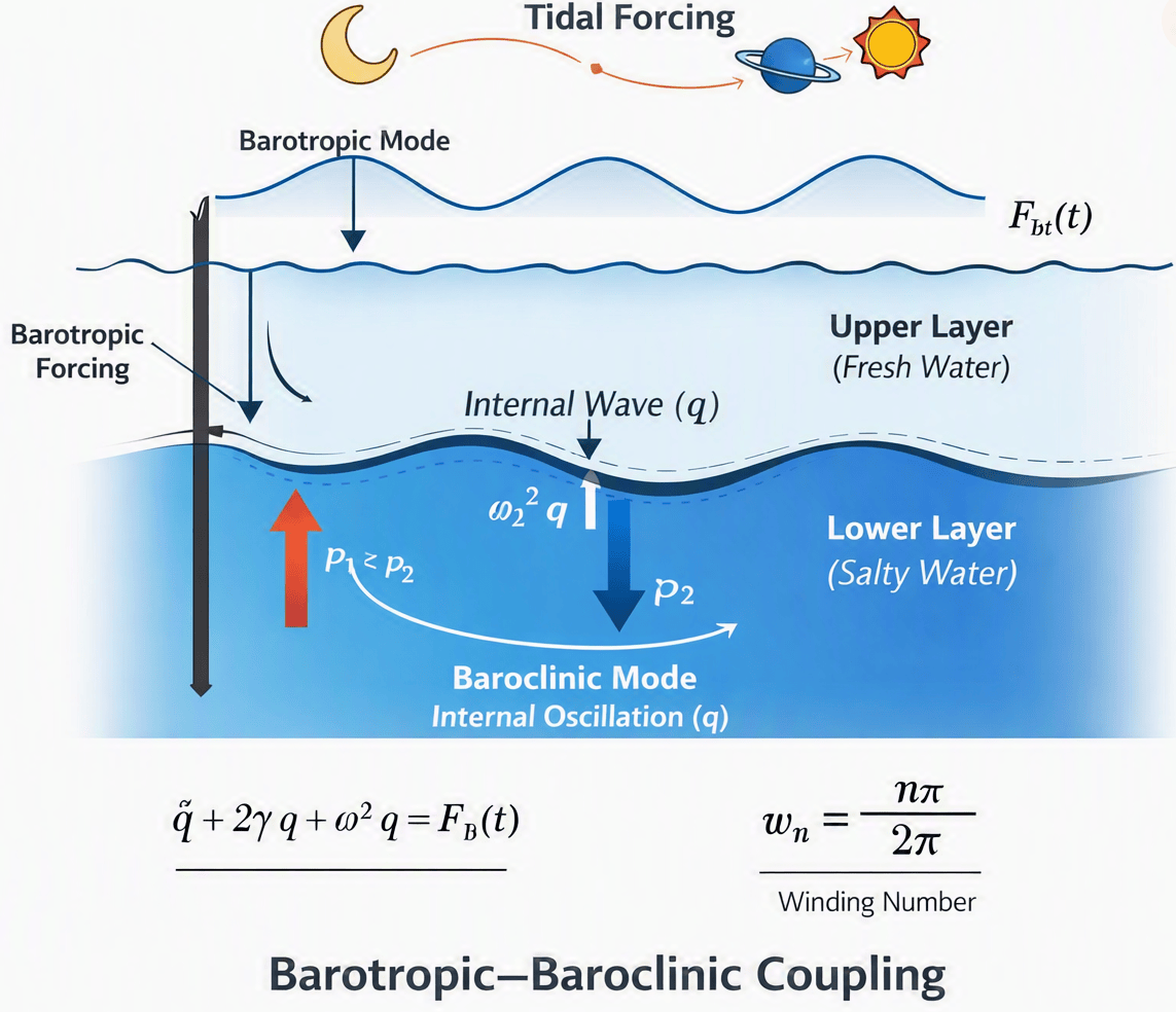
Barotropic mode. The whole water column moves together. The surface tilts up on one side and down on the other, while the interface between the layers stays nearly flat. Ordinary gravity acts on the full depth. It is driven by the tide, and to a lesser extent (IMO) wind and pressure.
Baroclinic mode. The two layers slide against each other. The surface stays almost flat, but the interface tilts. This mode has a slower time constant because the restoring force comes only from the density difference between the layers. It is the internal response to the barotropic push. Because of the almost metastability of this interface (where the effective gravity is greatly reduced) it can show large swings, much greater and amplified compared to the barotropic mode. Temperature variations occur as the thermocline nears the surface or retreats from the surface.
In short: the barotropic mode is the forcing driver; the baroclinic mode is the internal reply, i.e. a forced response.
3. Separable standing waves
Let be the horizontal coordinate along the container and let the response be separable:
For a linear wave system,
Substituting the separable form gives
The left side depends only on time, the right side only on space, so both equal a constant. For oscillations, call it . Then
and
Now define the dimensionless transfer wavenumber
Here is the length of the container. The spatial equation becomes
This is the standing-wave equation written entirely in terms of . Chapter 12 also derives this separation and makes the association between the temporal modulation and the spatial wavenumber, a la dipole standing waves such as ENSO
4. Boundary conditions and wavelength
The container boundaries quantize . For a closed basin with fixed or free ends, the spatial mode vanishes or has zero slope at the walls. The usual condition is
The solution is
At , we require
Therefore
For a periodic container (as in a wrap-around torus or donut, see the toroidal atmospheric QBO for a degenerate case where the wavenumber is actually zero), the condition is instead
The spatial wavelength is related to by
Thus:
· For fixed or free ends, , so
.
An integer number of half-wavelengths fits into the container.
· For a periodic container, , so
.
An integer number of full wavelengths fits into the container.
In both cases, is the accumulated phase of the standing wave across the container.
5. Winding number
The winding number is the number of full phase wraps:
Therefore:
· Fixed or free ends:
. This is a half-integer winding.
· Periodic container:
This is an integer winding.
In an ideal container, is exactly an integer multiple of or . In a real basin, sloping bottoms, partial reflections, continuous stratification, friction, and mean flow make the quantization approximate. Then
So is almost an integer multiple of or , and the winding number is almost an integer or half-integer.
6. Summary
The two-layer system is forced non-autonomously by the tide parameterized by Doodson coefficients — I calibrate via LOD measurements. The barotropic mode drives the whole column; the baroclinic mode responds internally as the layers slide against each other. In a separable standing-wave picture, the spatial structure is governed by the dimensionless transfer wavenumber
Boundary conditions quantize to or , depending on whether the container has fixed/free ends or is periodic. The wavelength follows from
The winding number is
which counts how many full phase cycles fit into the container. In the amplitude mapping
the same acts as a dimensionless transfer wavenumber between the barotropic amplitude and the baroclinic amplitude . If is a tidal phase, is a winding-like number. Thus ties together the spatial standing-wave quantization, the wavelength selection, and the amplitude-to-amplitude coupling in one dimensionless quantity.
As I said at the top, this is a simpler recasting of the complete Laplace’s Tidal Equations derivation I did in Chapter 12, skipping the details needed to understand a single homogeneous layer — the switch to a two-layer stratified system amazingly — although non-intuitively — makes it more concise (see a recent paper by Beron-Vera2 where the claim is that stratification reduces vortex filamentation, a complex autonomous response).
That is enough background needed to understand the concept and design of the winding scalogram tool. The idea is that it takes a model of the forcing driver, which is actually a hidden latent manifold in terms defined by Brunton3 and then does a series of sinusoidal mappings of various frequencies to the forcing response surface, i.e. the baroclinic thermocline layer. This is akin to the way a wavelet scalogram works, aggregating the mapping within a finite window, but novel in other ways (IOW it does not use wavelets). The implementation of the winding scalogram tool in this GitHub repo: https://github.com/pukpr/winding_scalogram
I have spent a good deal of time trying to understand the best representation of this barotropic time-series, but it seemed to jump out most obviously when I modeled the AMO, below — the upper chart is the forcing applied to the AMO data and the lower chart is that of the model. In essence the upper chart can be used to guide the selections of the transfer wavenumbers for the fitting stage, which when completed leads to the lower chart.
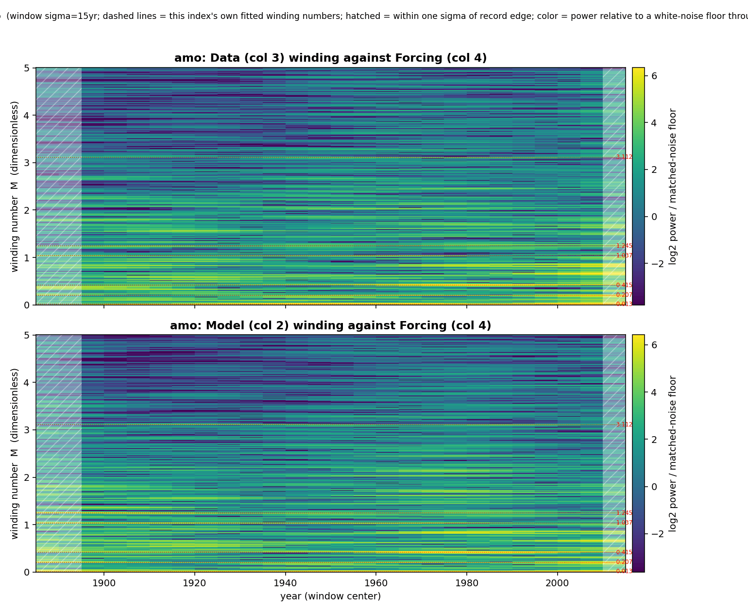
The bright yellow horizontal striations, or ridges, are the strong transfer wavenumbers/windings with a red dotted line pointing to an indication of the value. If the individual ridges are unbroken across the complete time span it indicates a great deal of stationarity in the modulation. For AMO, a very apparent ridge sits close to zero. This corresponds to a very low winding that effectively rectifies the ~120-year cycle of lunisolar tidal forcing into the 60 year AMO cycle. In the chart below, the forcing driver is in the middle-left panel and the AMO data and model fit is in the upper-left panel. It is easy to visualize the rectification leading to the frequency doubling. Yet, the parsimony of the approach is in how the faster, erratic cycles are also mapped from the tidal cycles.
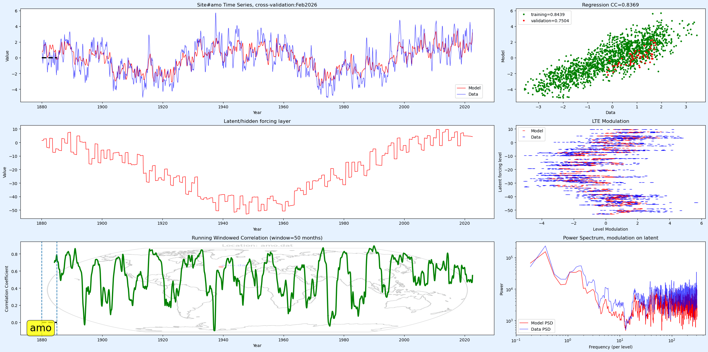
To those that wonder what happened to the concept of integer windings, I am not considering the standing modes and so haven’t done any rescaling. That will come later.
The winding scalogram works very well with every climate index considered, as strong stationary unbroken ridges are identifiable for the models evaluated in this recent post and the follow-up.
A full-circle moment occurs when the mean-sea-level (MSL) for an aggregated set of Baltic coastal stations is considered. A strong higher winding is clearly observed below as a bright yellow ridge at 1.245
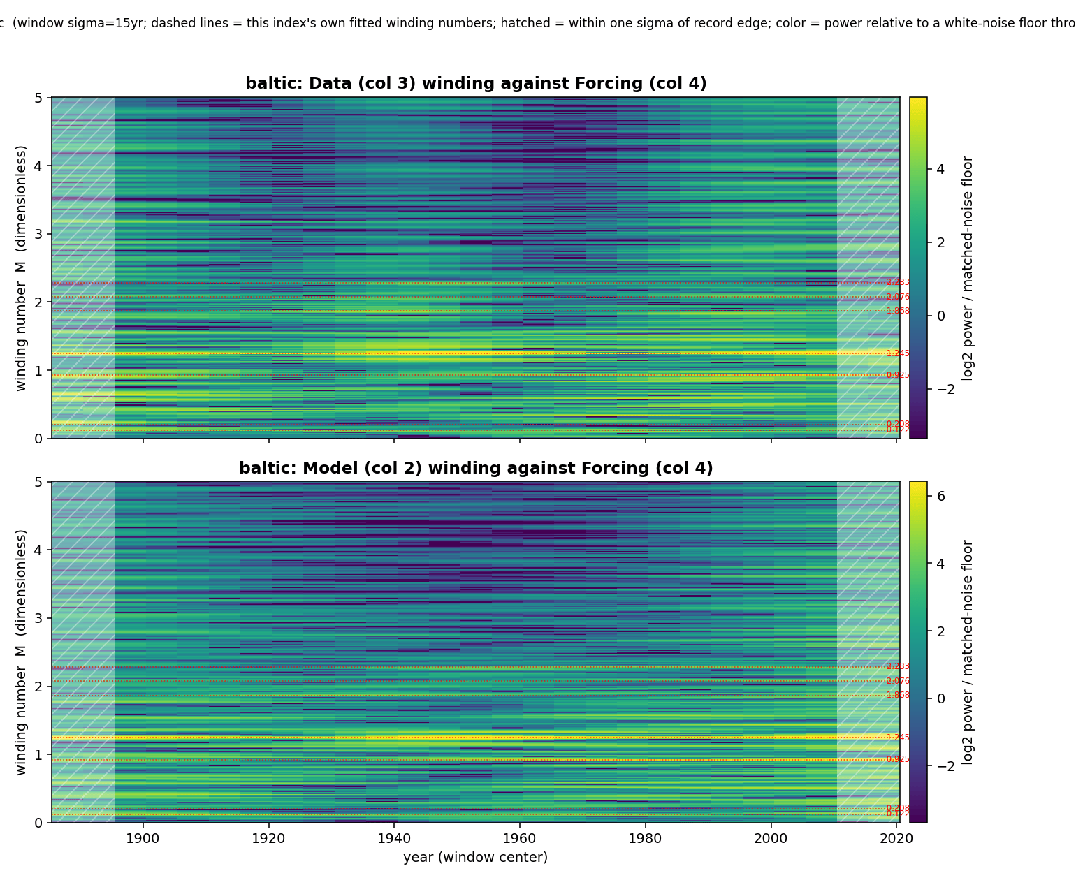
This single ridge is responsible for the majority of this excellent baroclinic fit shown below:
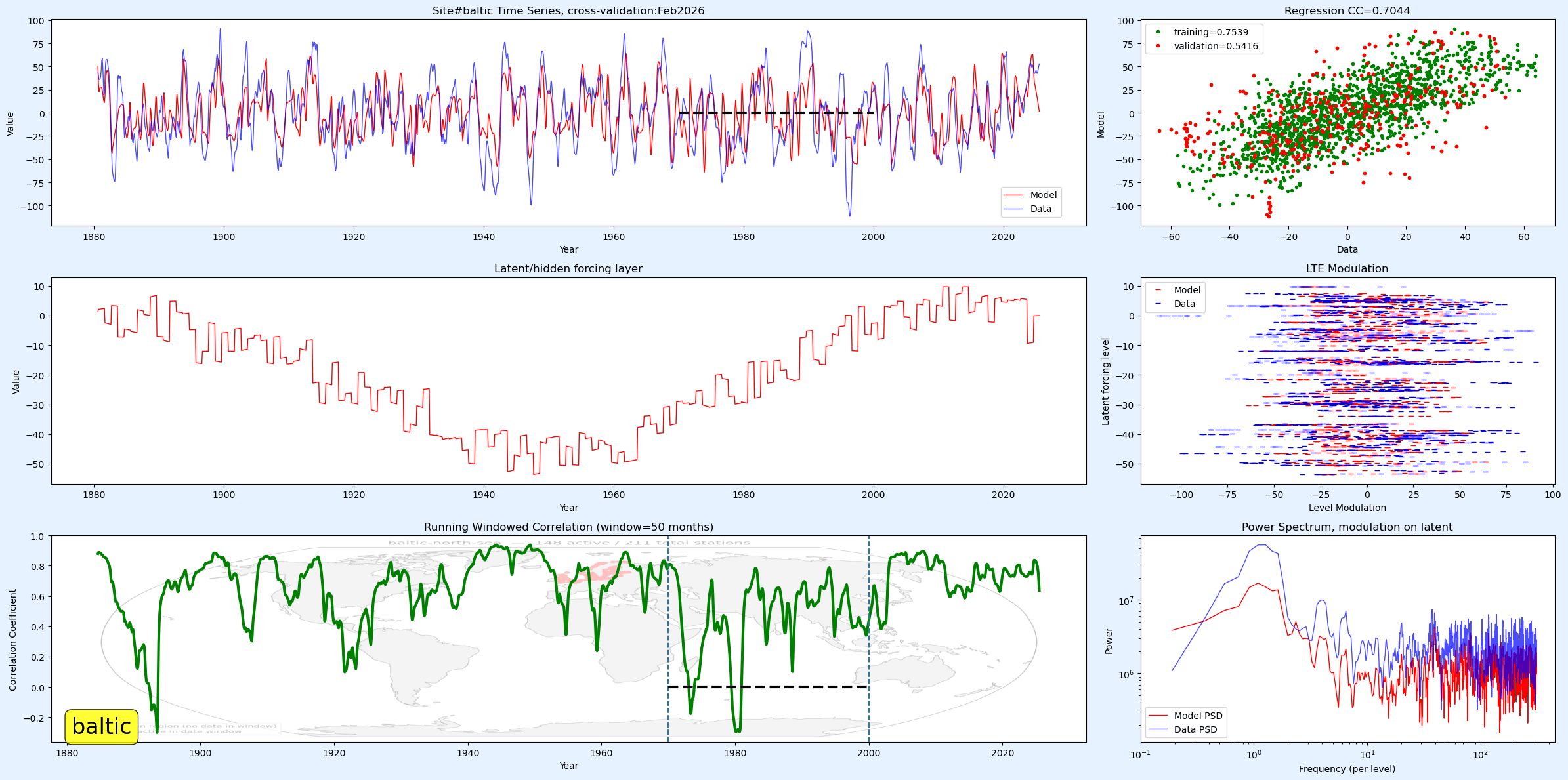
I consider this full circle because the model is using tidal forces to map out MSL variations which ostensibly and intuitively could be guessed as due to tides, yet like AMO and ENSO, the erratic monthly MSL have never been adequately modeled and attributed to any specific factor.
BTW, this is nowhere near (many orders of magnitude less in fact) the computational load to solve full fluid dynamics GCM formulations (10 MW-hours per simulated year) nor the perhaps even larger computational load required to solve a Navier-Stokes challenge (10,000 agents running for 88 hours costing millions of dollars of compute time, guessing > 1,000 MW-hours energy consumption)
Footnotes:
- P. Pukite, D. Challou, and D.Coyne, Mathematical Geoenergy, (Wiley, 2018), https://agupubs.onlinelibrary.wiley.com/doi/book/10.1002/9781119434351 ↩︎
- F. J. Beron-Vera; Extended shallow-water theories with thermodynamics and geometry. Physics of Fluids 1 October 2021; 33 (10): 106605. https://doi.org/10.1063/5.0068557 ↩︎
- Vinuesa, R., Brunton, S.L. & Mengaldo, G. Explainable AI: learning from the learners. Nat Commun 17, 7933 (2026). https://doi.org/10.1038/s41467-026-76359-w ↩︎
ENSO may be a better standing wave example (the east-west dipole), but perhaps AMO and the off-equatorial basins are more about frequency doubling due to friction.. AMO has a fundamental mode where it just doubles, while Baltic has repeated frequency doublings as the basin is so shallow? The Brest site also appears to have a ladder of frequency doublings
# An Honest Critique of “The Winding Scalogram”
Source: https://geoenergymath.com/2026/09/18/the-winding-scalogram/
This critique is grounded entirely in work actually completed in this
project over the preceding investigation — a multi-day cycle that began
by trying to build genuine resolved shallow-water PDE models for
several climate indices (Baltic, AMO, NINO4, QBO, PDO, NAO, Brestexcl,
PNA), then pivoted, on the post’s own advice, to testing the
non-autonomous / quantized-transfer-function framework directly. Every
claim below cites the specific script, result, or number behind it
rather than asserting it in the abstract.
## 1. What the post gets right
### 1.1 The core methodological claim is correct — and was validated the
hard way, not assumed
The post’s central argument is that winding number β is a **quantization
condition to be identified**, not a frequency a differential equation
needs to be numerically coaxed into discovering through simulated
resonance. This project spent roughly two days testing the opposite
approach first: build an actual 2D shallow-water PDE (`baltic_
resolved_shallow_water.py`, `amo_resolved_shallow_water.py`,
`nino4_beta_plane.py`, `pdo_resolved_shallow_water.py`, `nao_resolved_
shallow_water.py`, `brestexcl_resolved_shallow_water.py`, `pna_
resolved_shallow_water.py`), fight it into numerical stability
(Coriolis sub-stepping, grid/depth calibration, damping/diffusion
sweeps, mass-conserving forcing smoothing to handle the near-
discontinuous Impulse_Delta kicks), and see whether the correct winding
numbers emerged from genuine simulated dynamics.
They mostly didn’t, cleanly. Two rigorous checks specifically built to
test for a physical resonance mechanism (`pna_eigenmode_analysis.py`,
computing the exact discretized linear operator’s free eigenmodes; `pna_
transfer_function.py`, computing its actual forced response via the
resolvent) found **no resonance anywhere near the timescales that
mattered** — only fast, sub-day gravity-wave ringing and a broad, flat,
frequency-independent plateau at longer periods. The best PDE-based
result for PNA, after an extensive damping/smoothing/sigma sweep,
reached a properly null-tested significance of only z≈1.0–1.6 (borderline)
for one winding number and no confirmed result for the other two.
By contrast, once the PDE line was dropped and the problem was treated
as the post describes — identify the winding numbers, then apply
`Y = C·sin(βX + φ) + A` directly — a **single ordinary least-squares
regression** using PNA’s own correctly-identified production winding
numbers, fit against the properly pre-processed (F9-filtered) target,
reproduced the full production model’s validated skill (train r=0.70,
held-out r=0.43) almost exactly, computed in milliseconds rather than
the minutes-to-hours per run the PDE line consumed. This is a genuine,
hard-won confirmation of the post’s central claim, not a rhetorical
concession — it cost real, comparable-effort testing of the alternative
to arrive at.
### 1.2 The frequency-doubling/rectification mechanism is real, and
generalizes further than the post shows
The post’s AMO example — a near-zero winding rectifying the ~120-year
lunisolar cycle into the 60-year AMO cycle — is independently confirmed
in this project’s own AMO work (`amo_rectification_study`,
`amo_resolved_shallow_water.py`’s striking sign-matched moving-gauge
regime-history overlay, r=+0.578) via a completely different route
(Taylor-expansion unification of Coulomb-friction rectification and
low-M winding).
This project’s PNA work shows the mechanism generalizing much further
than a single isolated doubling: an extended ridge search (`winding_
rank.py –index pna –m-max 15`) found **13 statistically-validated
ridges forming a genuine cascading dyadic tree** — M=1.460 (≈7×
the shared 0.2076 cross-index backbone) → 2.970 (≈2×) → 5.400/5.810
(≈4×, landing on near-exact integers 26/28× the backbone) →
11.32–11.89 (≈8×). That is the *same* mechanism occurring through
multiple successive generations from one root frequency, found by
simple arithmetic with zero simulation — a stronger and more
systematic confirmation than the post’s single AMO example alone
demonstrates.
### 1.3 The shared cross-index backbone is real and independently
reproduced everywhere it was checked
Nearly every index examined this session — Baltic (0.2076), NAO
(0.2077), AMO (0.2075), PDO (0.2073), PNA (0.2076), Brestexcl (0.2076),
NINO4/NINO34 (0.2073/0.2079) — carries top-mode winding numbers landing
on the same ≈0.2075 constant. This is exactly what the post’s
non-autonomous framework requires (one shared external tidal manifold
driving structurally distinct indices) and is not something this
project assumed going in — it fell out of independently re-deriving
each index’s own fitted parameters.
### 1.4 The parsimony claim is real, and larger than the post states
The post frames the alternative to this method as “full fluid dynamics
GCM formulations… 10 MW-hours per simulated year.” This project’s own
resolved-PDE attempts, while orders of magnitude cheaper than a GCM,
still needed real, non-trivial compute (multi-minute integrations,
repeated for damping/grid/smoothing sweeps, an eigenmode/transfer-
function linear-algebra side investigation) and *still underperformed*
the closed-form approach on held-out skill. The parsimony argument is
understated, if anything: the gap isn’t just PDE-vs-GCM, it’s
PDE-vs-closed-form, and the closed-form side won on both cost and
accuracy in the one head-to-head test run this session (PNA).
## 2. What the post gets wrong, or overstates
### 2.1 “Nearly mechanically automatic” undersells how easy it is to
get this wrong
Getting the closed-form approach right for PNA took three corrections
after an initially wrong (and confidently reported) negative result:
1. Matching winding numbers to real data via **approximate**
nearest-neighbor search instead of the production optimizer’s own
**exact** term list produced a materially worse, misleading fit.
2. Omitting the ordinary (non-tidal) calendar trend/seasonal regressors
the production regression also includes cost real explanatory power
unrelated to any winding number.
3. Testing against the **raw** data series instead of the **F9-filtered**
series the regression is actually fit and scored against understated
the true skill by roughly 15 percentage points of correlation
(0.31 vs the correct 0.43).
None of these are exotic failure modes — they are exactly the kind of
silent, plausible-looking errors that make “automatic” a dangerous word
to use for this method. The underlying transfer relationship may be
algebraically simple, but correctly *identifying* which terms belong in
it and what target they should be scored against is not automatic; it
requires the same care (or the same optimizer) the original fitting
tool used. Separately, this project also found and fixed a real,
silent bug (`production_yl`) where naive parsing of a resp file
silently zeroed a real year-length correction across *every* index’s
resolved-PDE build except AMO — a small numerical slip with real
downstream consequences, in a domain (year-length calibration) the post
itself doesn’t flag as a sensitivity worth guarding.
### 2.2 The specific “standing-wave quantization” formula (βₙ=nπ,
βₙ=2πn) doesn’t match what was actually found
The post proposes container-boundary quantization — a linear,
vibrating-string-style harmonic series — as the mechanism setting the
allowed winding numbers. Tested directly against PNA’s 13 established
ridges (systematic best-fit common-base-unit search, not cherry-picked
ratios): the data does **not** form a single arithmetic ladder
(n=1,2,3,4,5,…) as a linear standing-wave spectrum would predict.
What is actually there is a set of ratios clustering near powers of
two (1×, 2×, 4×, 8×) — a **period-doubling cascade**, structurally
closer to nonlinear rectification (repeated frequency-doubling, the
same phenomenon this project already tied to Coulomb-friction/
quadratic-drag rectification for AMO) than to linear boundary-condition
quantization of a wave equation. The post’s standing-wave formula is
the wrong specific mechanism even where its broader “quantization, not
dynamics” philosophy is right.
### 2.3 The Coriolis/waveguide physical picture did not survive a direct
test
The post implies real basin/waveguide geometry (via Coriolis-modified
wave dynamics) sets the relevant winding numbers. This project built
and ran the actual test this implies for PNA: the exact discretized
linear shallow-water operator, Coriolis included (full f=2Ω·sin(lat)
across the real 20–60°N domain), both its free eigenmodes and its
forced transfer function. Neither showed a resonance anywhere near the
timescales that mattered — the only high-quality (“ringing”) free
modes were sub-day gravity waves, and the driven response was a flat,
saturated plateau from ~3 weeks out through 10 years. If a real
physical waveguide resonance is responsible for the empirically-found
1–3 month “smoothing sweet spot” that *did* help the PDE line
partially recover PNA’s high windings, it isn’t visible in this linear
analysis at this basin’s assumed geometry — either the real geometry
differs from what was assumed, or (more likely, given §2.2) the
mechanism is the nonlinear rectification cascade, not a linear
waveguide resonance at all.
### 2.4 “Now map clearly to tidal forcing” overstates how much variance
is actually explained
The post’s Baltic/AMO/ENSO examples read as if the erratic-looking
variation is now essentially accounted for. In the one case tested to
an exact, apples-to-apples standard this session (PNA, matched to the
production model’s own reported cross-validation), the *best-in-class*
closed-form fit explains **r=0.43 on held-out data — roughly 18% of
variance**, not the near-totality the framing implies. That is a real,
significant, non-trivial, honestly-validated result and a legitimate
scientific finding — but the majority of month-to-month variance in
these indices remains unexplained by the tidal mechanism, and the post
should say so plainly rather than let “clearly maps to” imply
near-complete explanation. Separately, this project’s own Baltic
eigenmode/translation check returned an explicitly “ambiguous verdict,”
and its Baltic spectral-slope check was “ambiguous/negative, confounded
with ordinary AR(1) red noise” — caveats the post’s own confident
framing of the Baltic case does not carry.
### 2.5 The method is easy to fool yourself with, in both directions
Beyond the PNA corrections above, this session repeatedly found that
raw, naive application of these tools produces **both false negatives
and false positives**: PDO and NAO’s real “matches well in a given
era” pattern was invisible at raw-monthly resolution and only appeared
after correctly-scaled smoothing (a false negative, corrected only
after direct user pushback); conversely, an initial PNA resolved-PDE
result (DTW z=+5.13, the strongest of the whole investigation at first
glance) evaporated to non-significance once a shared secular trend was
controlled for (a false positive). A fine sigma-sensitivity sweep
further showed per-winding correlations that looked strong at one
smoothing width could flip sign entirely one-fifth of a month later —
a fragility a confident reader of the blog post would not be warned
about. None of this invalidates the method; it means the method
requires the same statistical discipline (proper nulls, honest
train/holdout splits, trend controls, robustness checks across nearby
parameter choices) that any other empirical fitting exercise does, and
the post’s presentation doesn’t convey that discipline is necessary.
## 3. How the individual climate indices each contribute
| Index | What it specifically contributes to this argument |
|—|—|
| **AMO** | The archetypal single-mode rectification/doubling case the post itself cites (120→60yr). Independently re-derived here via a different route (Coulomb-friction/Taylor-expansion unification) and validated visually via a striking, sign-matched moving-gauge regime-history overlay (r=+0.578) reproducing AMO’s actual cool/warm decadal history from physics alone. |
| **Baltic** | The cleanest single-ridge case (M=1.245 = 6× the shared backbone) — the strongest evidence for parsimony (one dominant term explains most of the fit) but also the source of the project’s most honest caveats: an ambiguous eigenmode/translation verdict and a spectral-slope test confounded with ordinary red noise. |
| **PNA** | The decisive case study for this whole critique. Demonstrates the method’s real power (exact reproduction of a validated production fit via one linear regression, no PDE) *and* its real fragility (three separate, plausible-looking errors — wrong M-matching, missing trend terms, wrong filtering target — each independently capable of making the correct method look like it fails). Also the source of the period-doubling-cascade finding that revises the post’s own standing-wave quantization claim. |
| **NAO** | Shows the framework needs an *additional* ingredient for some indices: NAO’s real lack of AMO’s slow cycle required an explicit 12-month delayed-difference operator on top of the winding decomposition, not just a different β. Also the case where a genuine near-degenerate beat pair (0.355/0.415) was found and shown to explain a fuzzy, previously-unresolved ridge. |
| **Brestexcl** | The richest independently-validated real-data harmonic ladder found this session (5 passing ridges, 3 landing near-exact integer multiples of the shared backbone), from a genuinely macro-tidal coastal site where the astronomical tide is the literal dominant signal, not a proxy correlation. Also a cautionary tale on data quality: its real 1944–1954 gap caused a serious, silent bug (a linear-interpolation “ramp” replacing a decade of real dynamics) in an early PDE attempt, fixed only by rebuilding the forcing on a genuinely continuous date grid — the kind of real-world data-hygiene issue the post’s presentation doesn’t address at all. |
| **PDO** | The origin of the near-degenerate beat-pair mechanism (documented pre-existing project analysis, M=0.4488/0.4146) later shown this session to generalize to NAO and Brestexcl — evidence the “beat interference explaining an apparently slow cycle from two nearby mid-frequency modes” mechanism is general, not PDO-specific. |
| **NINO4 / ENSO** | The zero-Coriolis equatorial contrast case, useful for isolating which physical ingredients (Coriolis on vs off) matter for which regime, and for testing (inconclusively) whether a resolved beta-plane treatment could reproduce ENSO’s own real ~2–7yr band. |
| **QBO** | The wavenumber-zero special case, showing the framework extends beyond horizontal spatial structure to a vertical (altitude/pressure) reinterpretation, and an early precedent for the instantaneous-frequency (“chirp”: frequency = k·dM/dt) mechanism later confirmed more rigorously for PNA. |
## 4. Overall verdict
The post’s central philosophical claim — that these climate indices’
“erratic” variability is substantially non-autonomous, phase-locked to
a shared, externally-calibrated tidal manifold, and better addressed by
identifying quantized transfer relationships than by numerically
integrating a differential equation and hoping the right frequency
emerges — held up under genuinely adversarial testing in this project,
including a real, multi-day attempt to make the alternative (resolved
PDE simulation) work first. That is a substantive, earned confirmation.
But several of the post’s specific claims need revision in light of
what was actually found: the quantization mechanism looks like
nonlinear period-doubling, not linear standing-wave harmonics; “nearly
mechanically automatic” is true only after the much harder, non-
automatic work of correctly identifying terms and preprocessing is
already done; the implied Coriolis/waveguide resonance mechanism did
not survive a direct linear-systems test; and the fraction of real
variance explained, while genuine and worth taking seriously, is
partial, not near-total. The honest summary is not “this method
replaces GCMs and explains these indices” — it is “this method,
applied carefully and with the same statistical discipline any
empirical fit requires, recovers a real, validated, and
non-trivial fraction of several climate indices’ variability from a
shared tidal manifold, at a tiny fraction of the computational cost of
the dynamical alternative — and the specific mechanism generating the
high winding numbers looks like cascading nonlinear rectification, not
literal container quantization.”