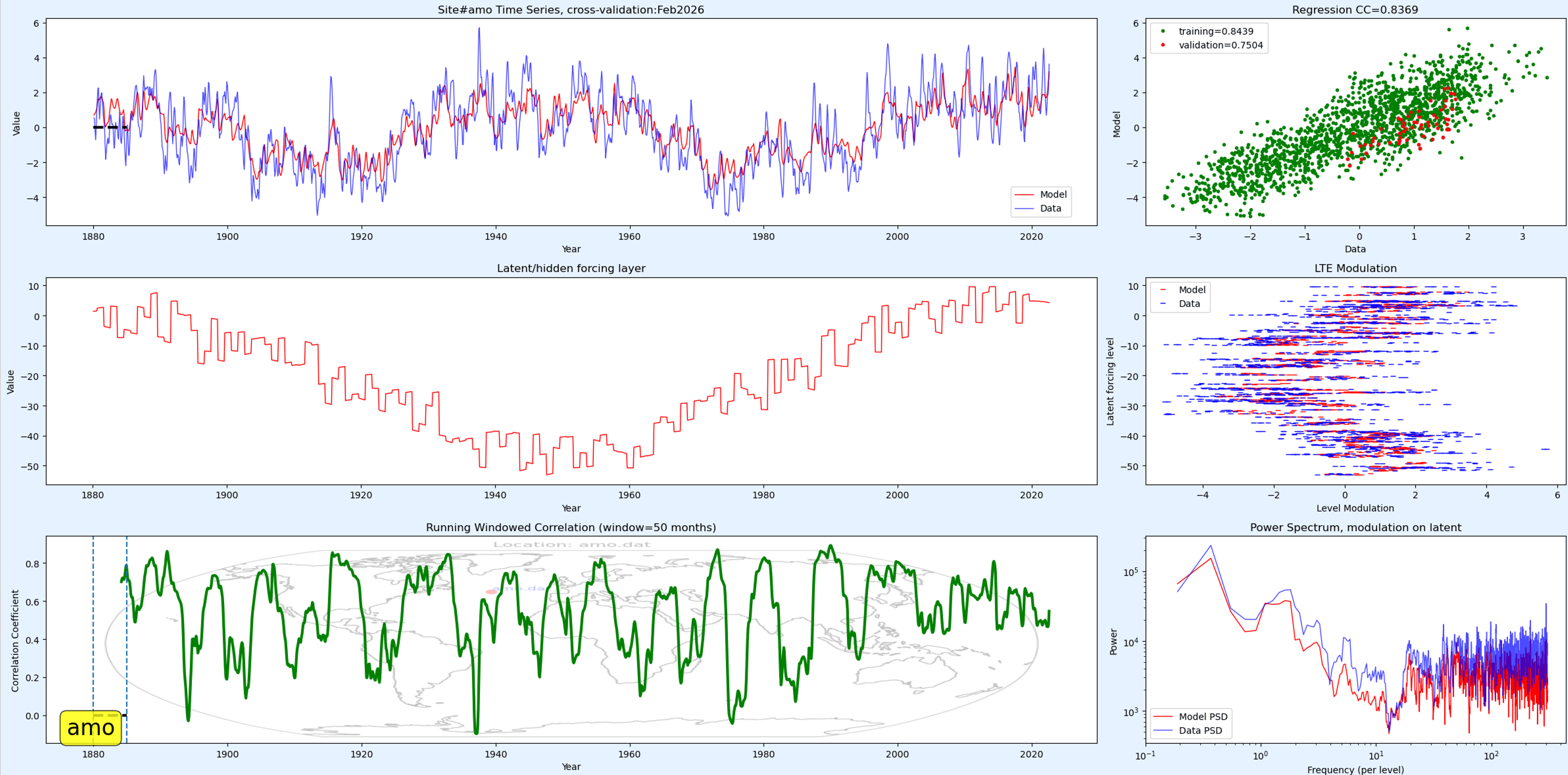
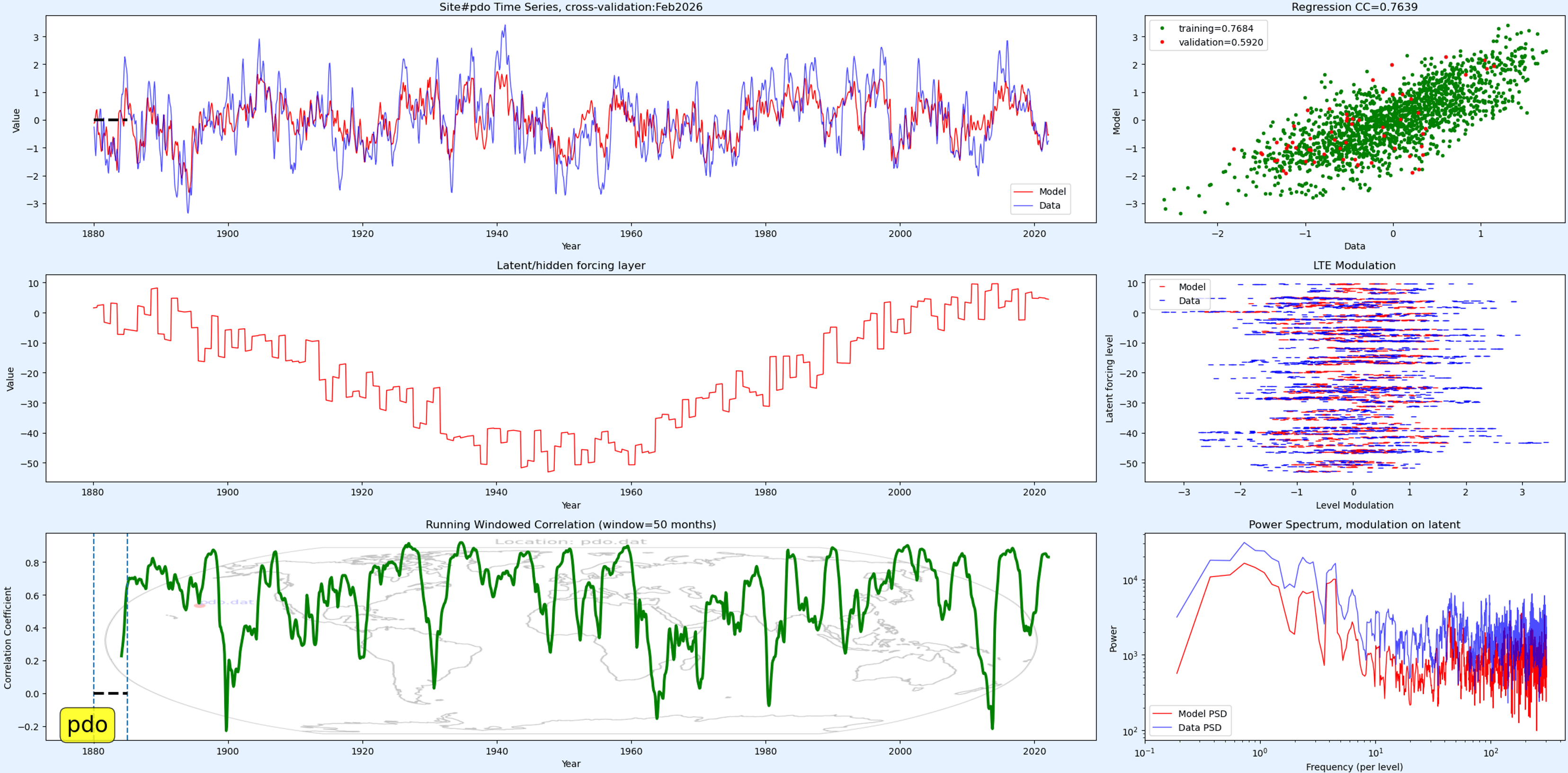
An algorithm that simultaneously optimizes the model fit to two disparate climate indices while keeping the hidden latent manifold constant. The two indices chosen, AMO and PDO, occur in separated ocean basins and show longer term variations, so that a multi-scale fit is necessary. The hidden latent manifold uses as a starting point the calibrated tidal factors needed to match the Earth’s LOD variations — the same torques that presumably cause the ocean’s thermocline to slosh. Only a slight perturbation to the tidal factors — amounting to a 0.996 correlation coefficient (instead of 1.0) to the calibrated LOD was needed to tweak the manifold during the fitting process.
AMO
PDO
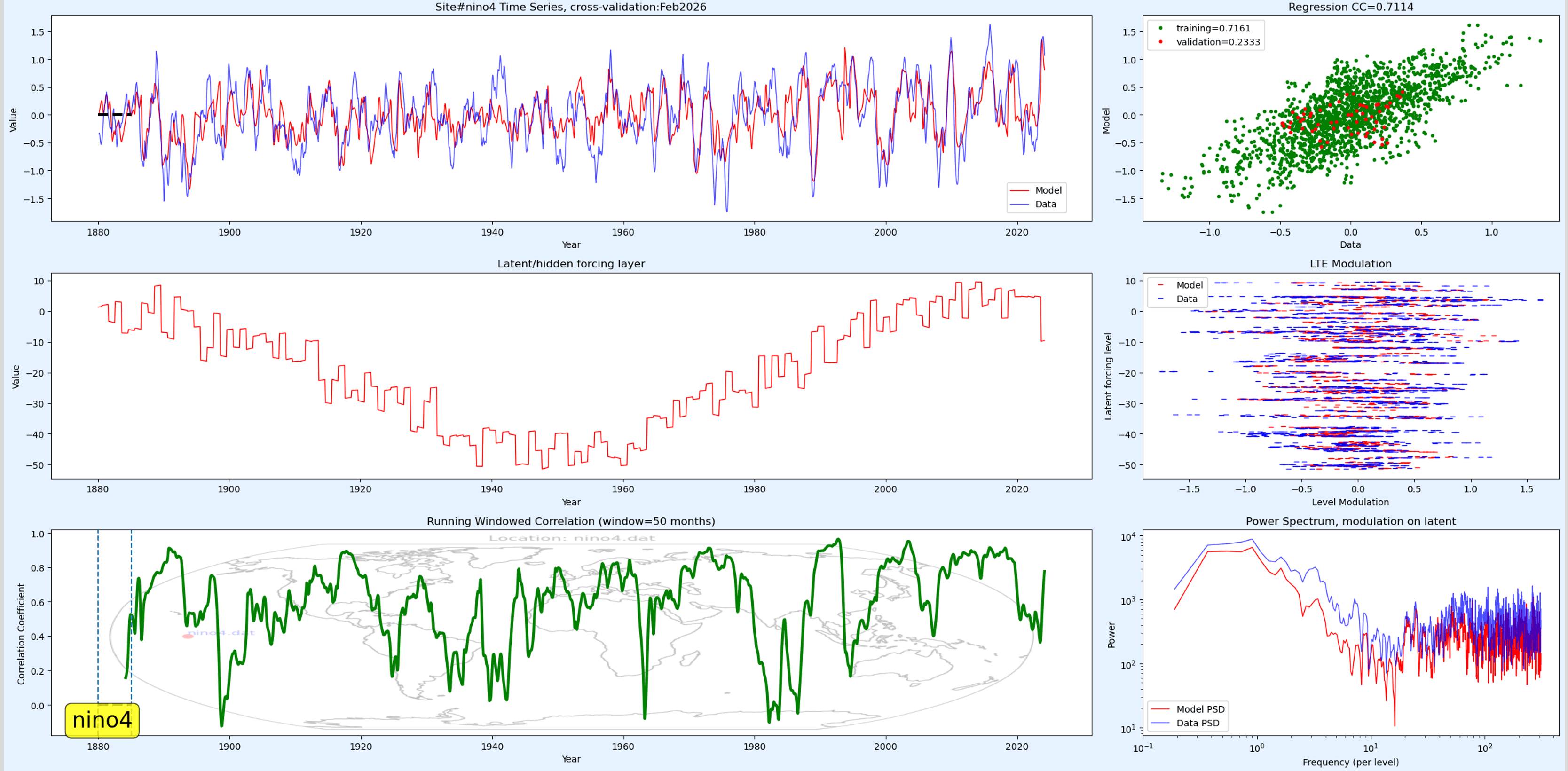
Can then use PDO as a seed to model NINO4 and IOD-East
NINO4
IOD-East
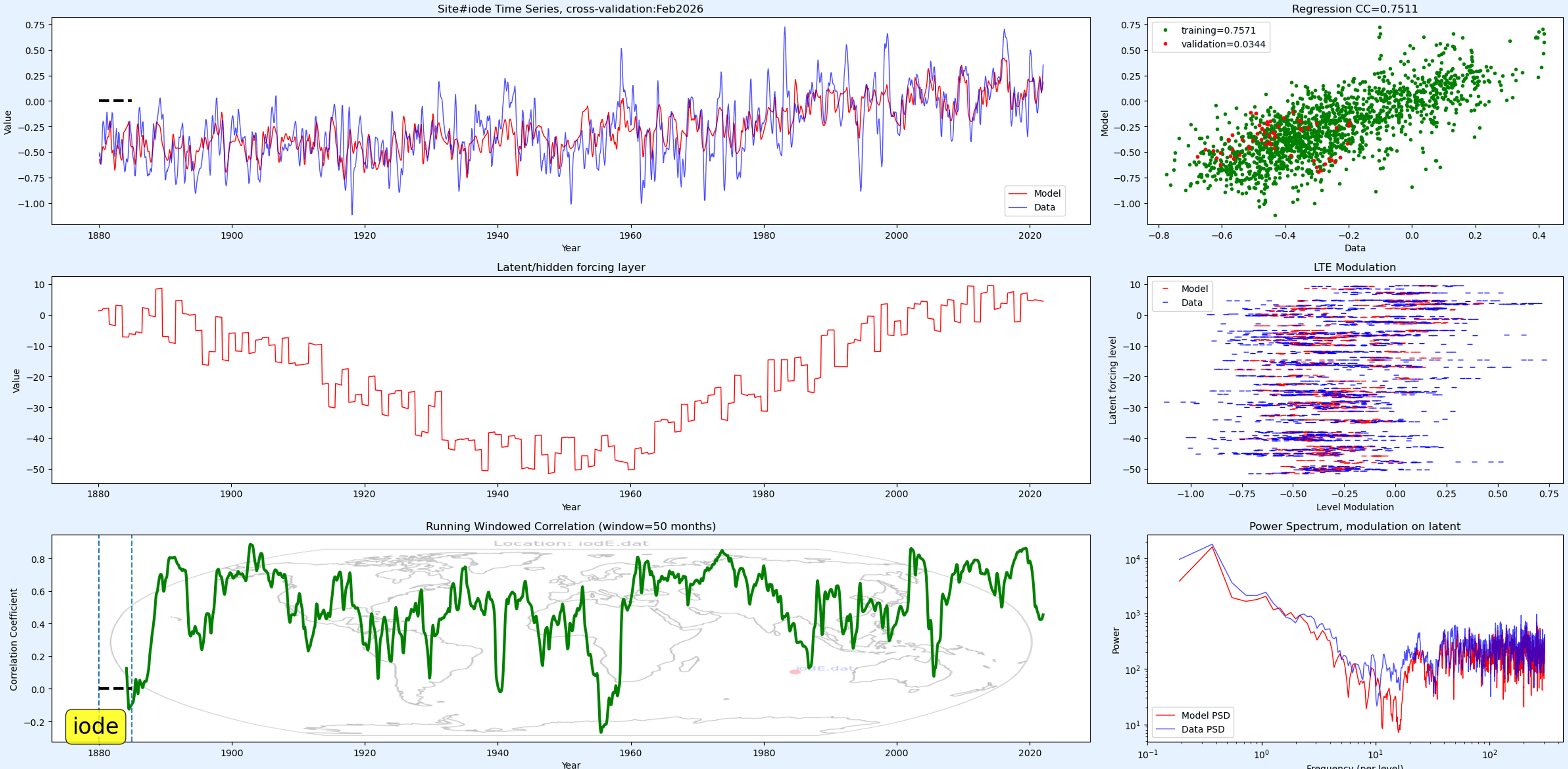
The manifolds are all aligned (below) with slight jogs that were caused by letting the fitting routine to proceed beyond the locked manifold stage.
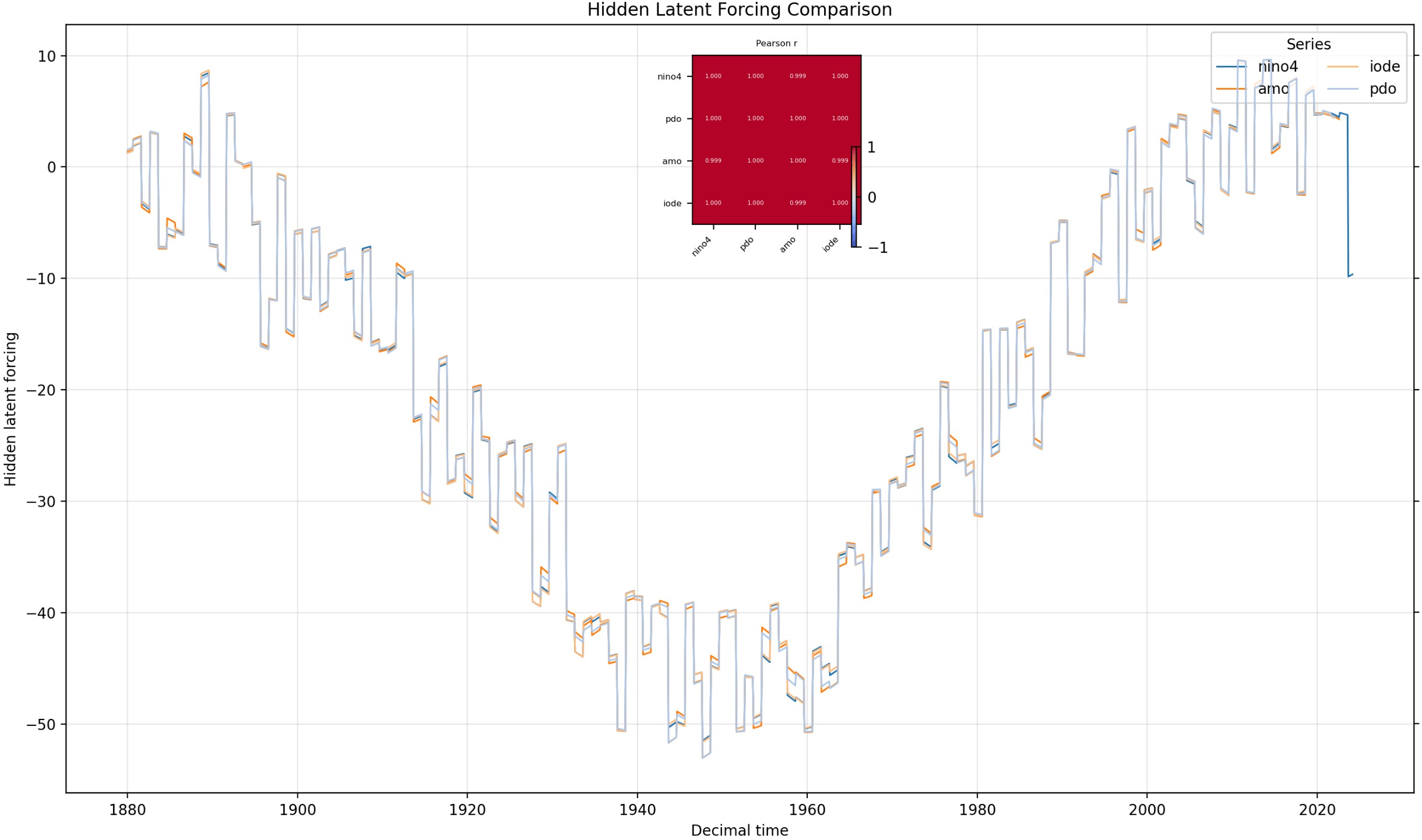
Have not included NAO in this set of comparisons yet since NAO has an interesting relationship to AMO. If the value of AMO from 12 months back is fed back into the current AMO with a negative sign (a delay differential), and then the correlation coefficient is computed, that value is significant, especially on more recent values.

The plot below is an expedited fit that does a delay differential on the AMO model to emulate the NAO time series. Note that the fit degrades in the years 1890-1900 and 1915-1920, the same years that the above pot shows anti-correlations.
NAO

Also averaged Baltic MSL time-series. Has a dominant LTE mode, higher in winding frequency than the other indices.
Baltic MSL

It is so strong that other LTE windings do not contribute much to the variation in extremes.
For PDO power spectrum, analyze the peaks in terms of harmonics. Also note the “flattened” shapes of the peaks. What can that be a result of — some distribution or non-stationarity in the spectral content?
KIMI response:
## Peak analysis (quantified by digitizing the plot)
Calibrating the log–log axes (ticks at 0.1/1/10/100; 10²/10³/10⁴) and tracing both curves pixel-by-pixel gives:
| Peak | Model (red) | Data (blue) |
|—|—|—|
| Low-freq complex | broad plateau ~0.4–1.0, crest ~0.73 | broader plateau ~0.35–1.0, crest ~0.73, extra shoulder ~1.8 |
| Mid peak | ~2.8 | ~2.34 |
| Strong peak | ~4.34 | ~4.39 |
| Peak | ~6.28 | ~6.28 (both curves agree exactly) |
| Strong peak | ~8.89 | ~8.89 (both agree) |
**Harmonic content.** The strong peaks are nearly exact doublings: 8.89/4.39 ≈ 2.03, and 4.39/2.34 ≈ 1.88. So the spectrum is a harmonic family — i.e., a non-sinusoidal, nonlinearly generated oscillation with a fundamental near **f₀ ≈ 0.7–1.1 per level**, with strong components near the 2nd/4th/8th multiples (a “dyadic” pattern typical of a relaxation-like or clipped waveform, or of a period-doubling structure where each doubling leaves a spectral line). The fact that model and data agree on 6.28 and 8.89 to within 1% says these are genuine deterministic harmonics, not estimation noise. Above ~30/level both spectra collapse into broadband noise, with the data carrying substantially more high-frequency power than the model.
## The flattened peak tops — what causes them
I measured the FWHM of each peak, and the diagnostic is striking:
– Peak at 0.73: Δf/f ≈ 0.45 (width ≈ 0.3 Hz)
– Peak at 2.8: Δf ≈ 0.7 Hz
– Peak at 4.3: Δf ≈ 0.65 Hz
– Peak at 6.3: Δf ≈ 0.6 Hz
– Peak at 8.9: Δf ≈ 1.0 Hz
**The absolute width in Hz is roughly constant across all harmonics, while the relative width shrinks as ~1/n.** That is the fingerprint of the frequency itself being uncertain, not the amplitude. Each harmonic n·f₀ rides on the same instantaneous fundamental, so if the fundamental wanders over a band of ±δf, every harmonic is broadened by the same absolute amount. Candidate mechanisms, in order of how well they fit:
1. **Non-stationarity of the oscillation frequency (frequency drift/jitter).** Over a long record, the PSD line is the time-average of a wandering line, i.e., the line gets convolved with the histogram of instantaneous frequency. A flat top specifically suggests the frequency spends roughly equal time everywhere in a band (slow modulation, near-uniform occupancy) — this is probably your “non-stationarity in the spectral content.”
2. **A distribution of natural frequencies (inhomogeneous broadening).** Since the x-axis is “per level,” an ensemble of levels/units each with a slightly different f₀ produces exactly this: each harmonic is an image of the *distribution* of fundamentals. A flat-topped line ⇒ approximately uniform detuning distribution; Gaussian jitter would give rounded (Gaussian) tops instead. The observed plateaus lean toward a broad, fairly flat distribution.
3. **Merged adjacent harmonics.** At low frequency the broadened lines overlap: the 0.4–1.0 “hump” is plausibly the fundamental, 2nd and 3rd harmonics fused into one plateau, with the visible ripple on top being the unresolved individual lines interfering. This naturally produces flat segments with small sawtooth wiggles, as seen.
What it is *not*: plain windowing/spectral leakage would give sinc-like scallops and would scale with record length, not show this clean constant-Δf behavior; and pure amplitude modulation would broaden lines proportionally to frequency (constant Q), which is the opposite of what is measured.
**Bottom line:** the comb structure says the latent signal is a coherent nonlinear oscillation (harmonics of one fundamental, with a suspicious octave-doubling pattern); the flattened, constant-absolute-width peaks say that fundamental is not fixed — either it wanders in time within your record, or you are averaging over a distribution of units/levels with spread natural frequencies (or both). Note also that the data peaks are systematically broader than the model’s, so the model underestimates this frequency dispersion, and it misses the excess broadband floor above ~30/level — both point to unmodeled latent variability. A useful check: recompute the PSD on shorter, overlapping windows; if the peaks sharpen into narrow lines as the window shortens, it’s non-stationarity (drift); if they stay broad at all scales, it’s a static distribution of frequencies.
Pingback: Introducing the Winding Scalogram: A Novel Analysis Tool
Pingback: Predicting PNA Patterns: Uncovering Hidden Climate Cycles