In our book Mathematical GeoEnergy, several geophysical processes are modeled — from conventional tides to ENSO. Each model fits the data applying a concise physics-derived algorithm — the key being the algorithm’s conciseness but not necessarily subjective intuitiveness.

I’ve followed Gell-Mann’s work on complexity over the years and so will try applying his qualitative effective complexity approach to characterize the simplicity of the geophysics models described in the book and on this blog.

Here’s a breakdown from least complex to most complex

1. Say we are doing tidal analysis by fitting a model to a historical sea-level height (SLH) tidal gauge time-series. That’s essentially an effective complexity of 1 because it just involves fitting amplitudes and phases from known lunisolar sinusoidal tidal cycles.

_{This image has been resized to fit in the page. Click to enlarge.}

2. The same effective complexity of 1 applies for the differential length-of-day (dLOD) time-series, as it involves straightforward additive tidal cycles.

_{This image has been resized to fit in the page. Click to enlarge.}

3. The Chandler wobble model developed in Chapter 13 has an effective complexity of 2 because it takes a single monthly tidal forcing and it multiplies it by a semi-annual nodal impulse (one for each nodal cycle pass). Just a bit more complex than #1 or #2 but the complexity already may be too great for geophysicists to accept, as the consensus instead argues for a stochastic forcing stimulating a resonance.

_{This image has been resized to fit in the page. Click to enlarge.}

4. The QBO model described in Chapter 11 is also estimated at an effective complexity of 2, as it is impulse-modulated by nearly the same mechanism as for the Chandler wobble of #3. But instead of a bandpass filter for the Chandler wobble, the QBO model applies an integrating filter to create more of a square-wave-like time-series. Again, this is too complex for consensus atmospheric physics to accept.

_{This image has been resized to fit in the page. Click to enlarge.}

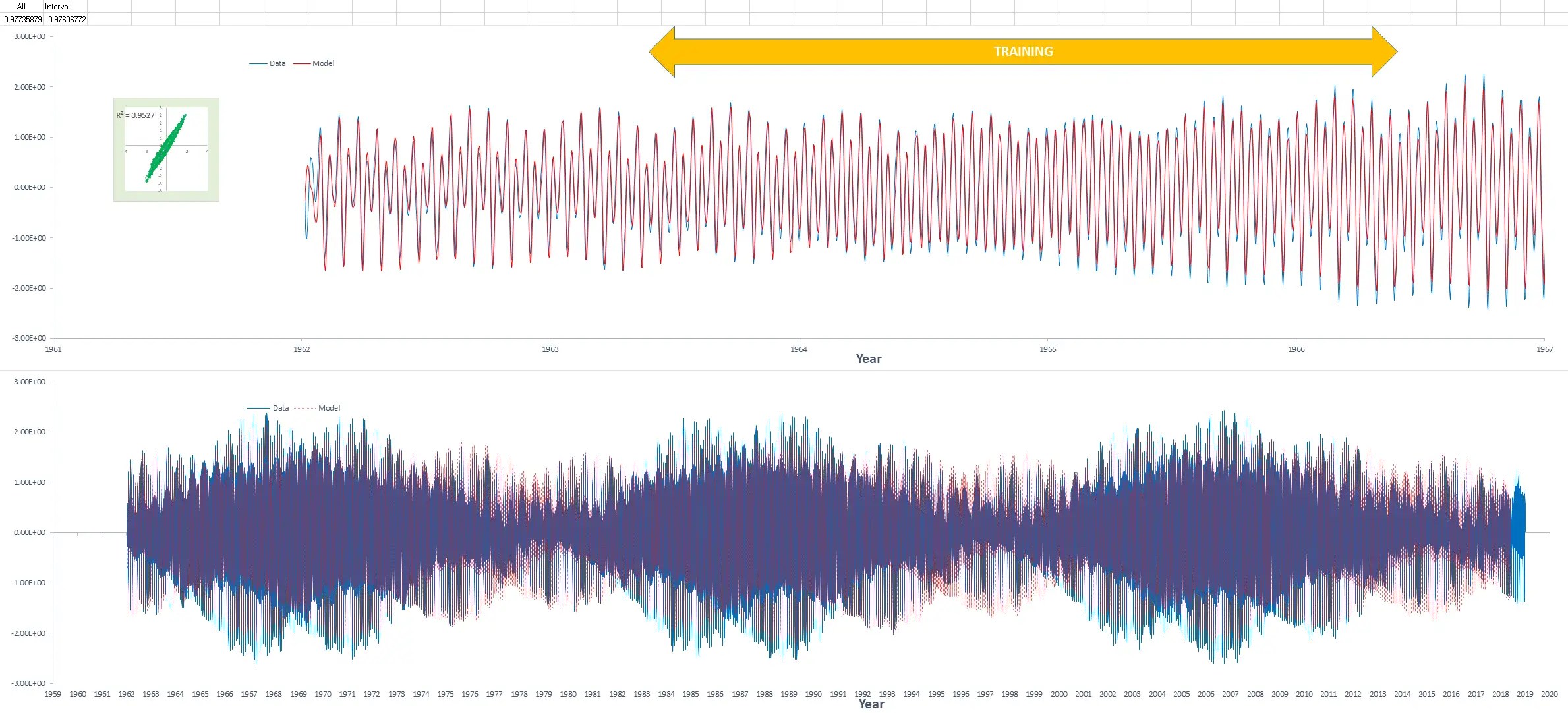
5. The ENSO model described in Chapter 12 is an effective complexity of 3 because it adds the nonlinear Laplace’s Tidal Equation (LTE) modulation to the square-wave-like fit of #4 (QBO), tempered by being calibrated by the tidal forcing model for #2 (dLOD). Of course this additional level of physics “complexity” is certain to be above the heads of ocean scientists and climate scientists, who are still scratching their heads over #3 and #4.

_{This image has been resized to fit in the page. Click to enlarge.}

The ENSO model is complex due to the non-linearity of the solution. The cyclic tidal factors can create harmonics from both the inverse cubic gravitational pull and from the LTE solution, and together with the annual impulse modulation creates an additional nasty aliasing that requires painstaking analysis to reveal.

By comparison, most GCMs of climate behaviors have effective complexities much more than this because — as Gell-Man defined it — the shortest algorithmic description would require pages and pages of text to express. To climate scientists perhaps the massive additional complexity of a GCM is preferred over the intuition required for enabling incremental complexity.

Since this post started with a Gell-Mann citation, may as well stick one here at the end:

“Battles of new ideas against conventional wisdom are common in science, aren’t they?”

“It’s very interesting how these certain negative principles get embedded in science sometimes. Most challenges to scientific orthodoxy are wrong. A lot of them are crank. But it happens from time to time that a challenge to scientific orthodoxy is actually right. And the people who make that challenge face a terrible situation. Getting heard, getting believed, getting taken seriously and so on. And I’ve lived through a lot of those, some of them with my own work, but also with other people’s very important work. Let’s take continental drift, for example. American geologists were absolutely convinced, almost all of them, that continental drift was rubbish. The reason is that the mechanisms that were put forward for it were unsatisfactory. But that’s no reason to disregard a phenomenon. Because the theories people have put forward about the phenomenon are unsatisfactory, that doesn’t mean the phenomenon doesn’t exist. But that’s what most American geologists did until finally their noses were rubbed in continental drift in 1962, ’63 and so on when they found the stripes in the mid-ocean, and so it was perfectly clear that there had to be continental drift, and it was associated then with a model that people could believe, namely plate tectonics. But the phenomenon was still there. It was there before plate tectonics. The fact that they hadn’t found the mechanism didn’t mean the phenomenon wasn’t there. Continental drift was actually real. And evidence was accumulating for it. At Caltech the physicists imported Teddy Bullard to talk about his work and Patrick Blackett to talk about his work, these had to do with paleoclimate evidence for continental drift and paleomagnetism evidence for continental drift. And as that evidence accumulated, the American geologists voted more and more strongly for the idea that continental drift didn’t exist. The more the evidence was there, the less they believed it. Finally in 1962 and 1963 they had to accept it and they accepted it along with a successful model presented by plate tectonics….”

https://scienceblogs.com/pontiff/2009/09/16/gell-mann-on-conventional-wisd

---

With all that, progress is being made in earth geophysics by looking at other planets. My high-school & college classmate Dr. Alex Konopliv of NASA JPL has lead the first research team to detect the Chandler wobble on another planet (this case for Mars), see “Detection of the Chandler Wobble of Mars From Orbiting Spacecraft” Geophysical Research Letters(2020).

In the body of the article, a suggestion is made as to the source of the forcing for the Martian Chandler wobble. The Martian moon Phobos is quite small and cycles the planet in ~7 hours, so this may not have the impact that the Earth’s moon has on our Chandler Wobble.

The wobble is small, about 10 cm on average.

Since a Mars year is 687 Earth days, only the 3rd harmonic (229 days) is close to the measured wobble of 206.9 days. With the Earth, it’s quite simple how the nodal lunar cycle interferes with the annual cycle to line up exactly with the Earth’s 433 day Chandler wobble (see Figure 3 up-thread in this post) , creating that wobble as a forced response, but nothing like that on Mars, which may be a natural response wobble.