In Chapter 12 of the book, we provide an empirical gravitational forcing term that can be applied to the Laplace’s Tidal Equation (LTE) solution for modeling ENSO. The inverse squared law is modified to a cubic law to take into account the differential pull from opposite sides of the earth.

The two main terms are the monthly anomalistic (Mm) cycle and the fortnightly tropical/draconic pair (Mf, Mf’ w/ a 18.6 year nodal modulation). Due to the inverse cube gravitational pull found in the denominator of F(t), faster harmonic periods are also created — with the 9-day (Mt) created from the monthly/fortnightly cross-term and the weekly (Mq) from the fortnightly crossed against itself. It’s amazing how few terms are needed to create a canonical fit to a tidally-forced ENSO model.

The recipe for the model is shown in the chart below (click to magnify), following sequentially steps (A) through (G) :

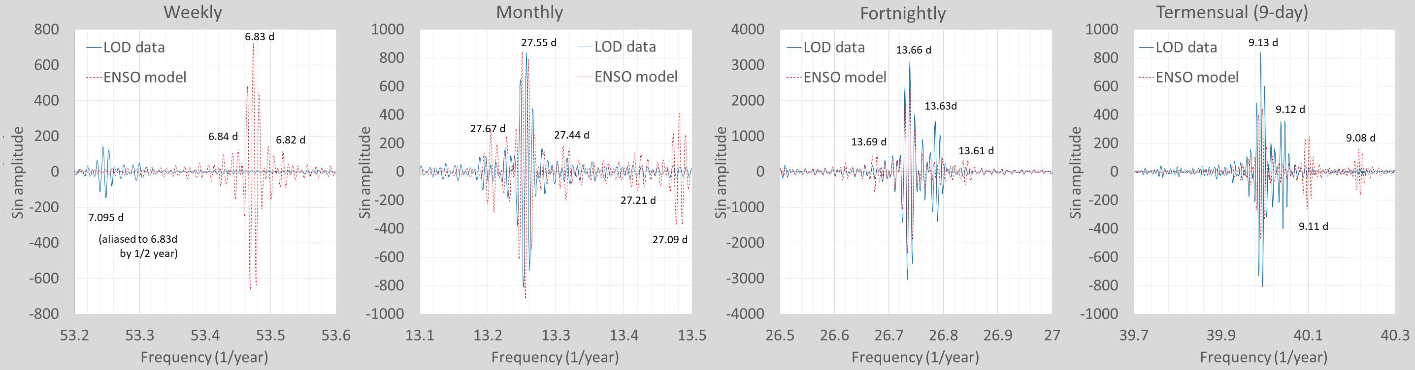
The tidal forcing is constrained by the known effects of the lunisolar gravitational torque on the earth’s length-of-day (LOD) variations. An essentially identical set of monthly, fortnightly, 9-day, and weekly terms are required for both a solid-body LOD model fit and a fluid-volume ENSO model fit.

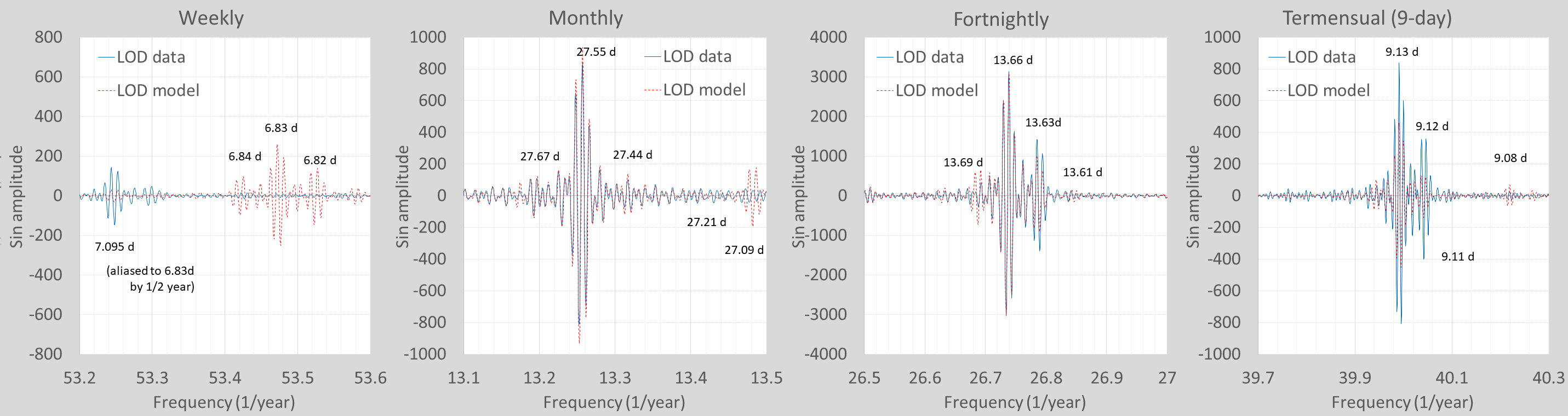
If we apply the same tidal terms as forcing for matching dLOD data, we can use the fit below as a perturbed ENSO tidal forcing. Not a lot of difference here — the weekly harmonics are higher in magnitude.

So the only real unknown in this process is guessing the LTE modulation of steps (F) and (G). That’s what differentiates the inertial response of a spinning solid such as the earth’s core and mantle from the response of a rotating liquid volume such as the equatorial Pacific ocean. The former is essentially linear, but the latter is non-linear, making it an infinitely harder problem to solve — as there are infinitely many non-linear transformations one can choose to apply. The only reason that I stumbled across this particular LTE modulation is that it comes directly from a clever solution of Laplace’s tidal equations.