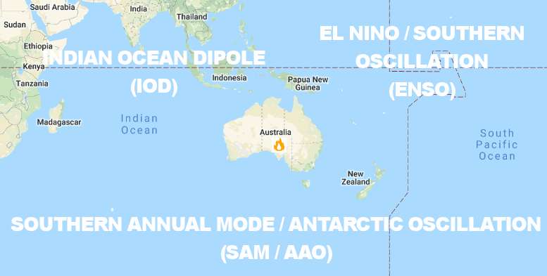
In Chapter 12 of the book, we focused on modeling the standing-wave behavior of the Pacific ocean dipole referred to as ENSO (El Nino /Southern Oscillation). Because it has been in climate news recently, it makes sense to give equal time to the Atlantic ocean equivalent to ENSO referred to as the Atlantic Multidecadal Oscillation (AMO). The original rationale for modeling AMO was to determine if it would help cross-validate the LTE theory for equatorial climate dipoles such as ENSO; this was reported at the 2018 Fall Meeting of the AGU (poster). The approach was similar to that applied for other dipoles such as the IOD (which is also in the news recently with respect to Australia bush fires and in how multiple dipoles can amplify climate extremes [1]) — and so if we can apply an identical forcing for AMO as for ENSO then we can further cross-validate the LTE model. So by reusing that same forcing for an independent climate index such as AMO, we essentially remove a large number of degrees of freedom from the model and thus defend against claims of over-fitting.
The new research on AMO by Professor Michael Mann appears to be meant to be somewhat provocative, which is OK as it spurred some discussion on Twitter. His peer-reviewed article is called “Absence of internal multidecadal and interdecadal oscillations in climate model simulations” and its takeaway is right in the title. Essentially, Mann et al are asking whether the ~60 year oscillation (and perhaps faster cycles) in the AMO behave as an internal property of the Atlantic ocean or whether the cycles are externally forced. Fig A1 in the Appendix provides some background on the AMO time-series data.
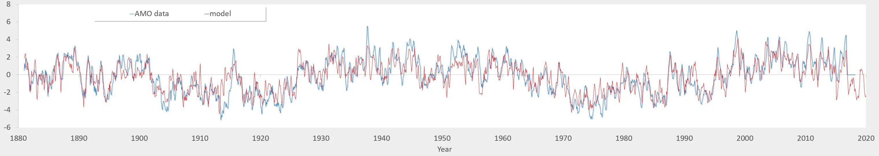
The characteristic of AMO that distinguishes it from ENSO is the multidecadal variation of ~60 years that it exhibits. In Fig 1 below, we show a model fit to AMO that relies on essentially the same input tidal forcing that was applied to the ENSO model. What is most impressive about the fit is how naturally the ~60 year cyclic variation emerges.
The comparison between the ENSO and AMO tidal forcing is shown in Fig 2 below. The clue to where the 60 year cycle arises from is in the slight modulated curvature in the profile.

What is causing the curvature is the interference between two closely aliased primary tidal forcings. These are the fortnightly tropical cycle of 13.66 days and the monthly anomalistic cycle of 27.55 days as described here in LOD characterization and see Fig A2 at the end of this post. These two, when interacting against a yearly annual impulse, produce a clear ~120 year repeat pattern as shown in Fig 3.

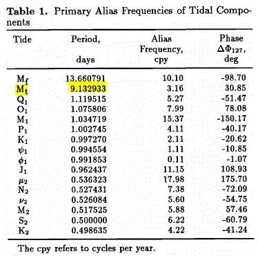
The two primary forcings acting mutually are also observed in tidal tables, in what is known as the long-period 9-day tide labelled “Mt” . From Fig 4 below the period of this tide is precisely 9.132933 days and so when applied to an annual impulse we get 365.242/ 9.132933 = 39.99175. This will reach a constructive interference against an annual impulse every 1/(40-39.9917)=121.3 years.
This value is important to consider for understanding how a ~60 year cycle comes about from the model. Since the LTE model is nonlinear, the 120 year underlying cycle can readily transform into a 60 year harmonic. Or these longer periods may not be as obvious, as with the ENSO model. So it just so happens that the 60 year cycle emerges in the AMO time series with the appropriate LTE modulation as in Fig 5 below (as it does with PDO).
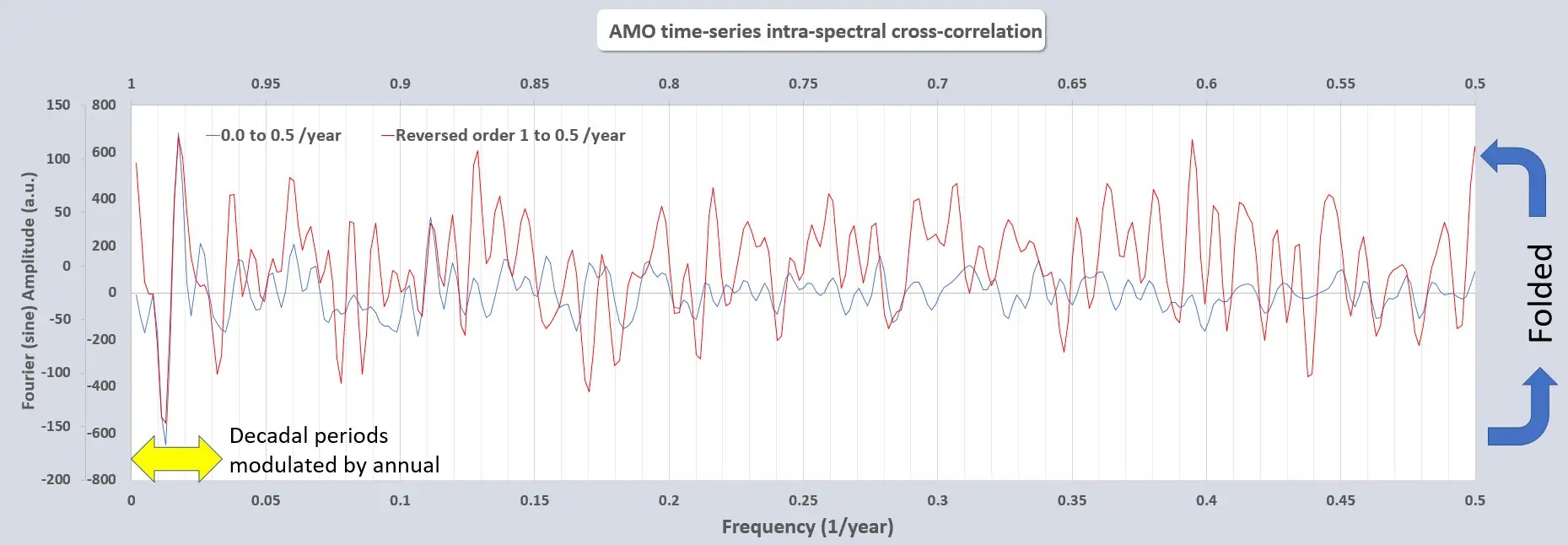
The 60 year modulation also appears as an intra-spectral cross-correlation as described in the previous post .
Furthermore, scientists at NASA JPL and the Paris Observatory have long known about a 60 year link between LOD and climate variation see Fig 6 below,.

The idea is that this multi-decadal period is integrated over time, creating a mutual interaction between the long-period forcing of the lunar + solar tides and the sloshing response of the ocean basins. The LOD or Universal Time (UT1) measure becomes a correlating measure of these forcing constituents. So the longer the period of potential constructive interference, such as with the 60 year near aliasing of the Mt constituent against a yearly impulse, the more that an inertial response can accumulate [4]. It may in fact be that the entirety of the LOD variations are due to the lunar + solar forcing and this is the unification between LOD and the climate dipole standing-wave behavior.

From [4]
References
- Cleverly, J. et al. The importance of interacting climate modes on Australia’s contribution to global carbon cycle extremes. Sci Rep 6, 1–10 (2016).
- Desai, S. D. & Wahr, J. M. Empirical ocean tide models estimated from TOPEX/POSEIDON altimetry. Journal of Geophysical Research: Oceans100, 25205–25228 (1995).
- Marcus, S. L. Does an Intrinsic Source Generate a Shared Low-Frequency Signature in Earth’s Climate and Rotation Rate? Earth Interact.20, 1–14 (2015).
- Dickman, S. R. Dynamic Ocean-Tide Effects On Earth’s Rotation. Geophysical Journal International, 112, 448–470 (1993).
Appendix
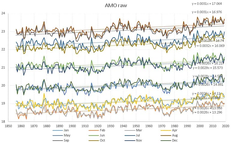
There is a strong annual component in the data as well as an increasing trend due to AGW– both of these are removed from the processed monthly data that we are fitting to.

Will do a similar post for PDO, here are the charts
Pingback: Tropical Instability Waves | GeoEnergy Math
Pingback: The PDO | GeoEnergy Math