I previously wrote about the Quasi-Biennial Oscillation (QBO) and its periodic behavior, and in particular how it interacts with ENSO — tentatively as a forcing. The ability of QBO to recreate the details of the ENSO behavior is remarkable. The possibility exists however that the forcing connection may be more intimately related to tidal torques which force QBO and ENSO simultaneously. Over a year ago, I first showed how the lunar tidal periods can be pulled from the QBO time series. See Figure 1 here, where the synodic month of 29.53 days is found precisely.
An interesting hypothesis is that the draconic lunar month of duration 27.2122 days may also be a common underlying significant driver. Unfortunately, the QBO and ENSO data are sampled at only a monthly rate, so we can’t do much to pull out the signal intact from our data … Or can we?
What’s intriguing is that the driving force isn’t at this monthly level anyways, but likely is the result of a beat of the monthly tidal signal with the yearly signal. It is expected that strong tidal forces will interact with seasonal behavior in such a situation and that we should be able to see the effects of the oscillating tidal signal where it constructively interferes during specific times of the year. For example, a strong tidal force during the hottest part of the year, or an interaction of the lunar signal with the solar tide (a precisely 6 month period) can pull out a constructively interfering signal.
To analyze the effect, we need to find the tidal frequency and un-alias the signal by multiples of 2π
So that the draconic frequency of 2π/(27.212/365.25) = 84.33 rads/year becomes 2.65 rads/year after removing 13 × 2π worth of folded signal. This then has an apparent period of 2.368 years.
This post will go into more detail and show how a combination of the synodic tide and draconic tide cycles are the primary forcers for QBO.
After reviewing some old Eureqa machine learning experiments on QBO, prompted by Graham at the Azimuth Project forum, I realized once again the significance of what it found. This is the learning recipe in 5 easy steps.
1. Started with raw QBO data

2. Next targeted a solution with sinusoidal factors
Set the fit criteria to maximize the correlation coefficient

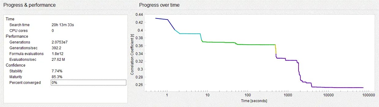
3. Then let Eureqa crank away
After 20 hours it looked like it wasn’t coming up with a better solution.
4. Picked a high complexity solution
The high complexity doesn’t really matter as the other solutions have similar common components.
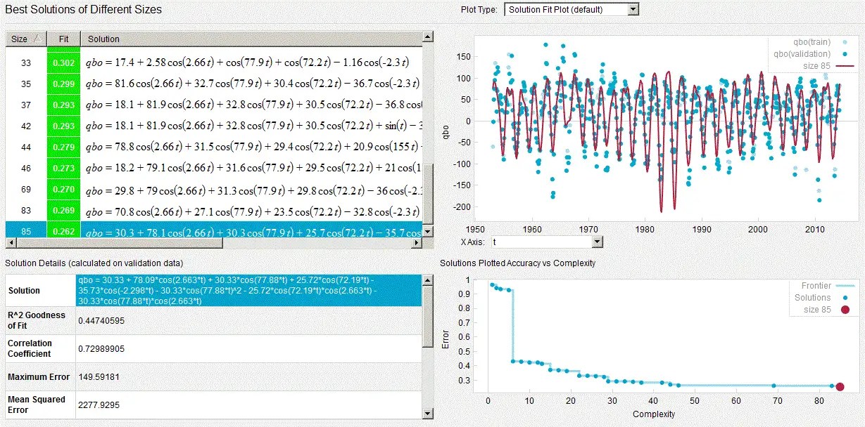
5. Focused on the two strongest factors that Eureqa found
These were sinusoids with an obviously folded or aliased frequency of between 2 and 3 years (i.e. quasi-biennial). The aliasing was obvious because it also selected high frequency components that, when folded, came out to the same 2 to 3 year period.
strength  aliased freq   period      in days          actual        % error
78         2.66341033   2.359075219  27.20894362  27.212=draconic  0.011233004
35         2.29753386   2.734751989  29.53743558  29.531=synodic  -0.021787874
6. The two factors have periods when un-aliased, match the Draconic and Synodic lunar month, with errors 0.01% and 0.02% respectively
What are the chances of that?
The results of the QBO characterization should not be surprising. The Wikipedia entry says that
” The precise nature of the waves responsible for this effect was heavily debated; in recent years, however, gravity waves have come to be seen as a major contributor and the QBO is now simulated in a growing number of climate models (Takahashi 1996, Scaife et al. 2000, Giorgetta et al. 2002)”
One form of gravity waves are the lunar tides, which happen to oscillate with the same frequency as QBO once the QBO signal is unaliased.
And that is likely the exact same mechanism for ENSO. The two behaviors, QBO and ENSO just happen to have the same underlying forcing mechanism. The numbers match up too well. The Baby D model of ENSO described in the previous post essentially includes the QBO as a forcing, but transitively this can be considered identically to applying the same synodic and draconic tidal forcing factor instead of the QBO !

Below is a simple model fit of the wave equation transformed SOI data. It uses the same strong Draconic and Synodic aliased periods as the QBO contains. I also included a periodic forcing of 2.9 years, which is the spin-orbit coupling oscillation of the Earth with the Moon [1].

I will try to automate this process and apply a least-squares fit ala the CSALT model and place it online via the Entroplet server.
Discussion
I am currently thinking that perhaps the ENSO and QBO are being forced by the same underlying factors, and what we are seeing with respect to the difference in the two responses results from the characteristics of the medium that generates the response. So that the QBO, characterized by a low density medium (thin air), is able to respond quickly and thus has a very high characteristic frequency. But the ENSO, characterized by the sluggish response of a huge volume of water operating on a thermocline, must have a much lower characteristic frequency. This lower characteristic frequency allows other factors, such as the Chandler Wobble and long-term tidal factors cycles to gain importance (essentially resonate more easily) and thus make the ENSO waveform much more erratic than the QBO. The latter essentially only responds to a narrow window of forcing between 2 and 3 years, so that that is why it looks much more periodic.
Please also read the commentary at the Azimuth Project Forum on evaluating the predictability of QBO.
As I said in a previous post, I was anticipating that the models for ENSO (and QBO) would be much more complex than they may have turned out to be. The mystery is why this simple forcing by tidal factors has escaped the notice of so many researchers over the years.
Perhaps they had seen it but thought it a coincidence. For me the plausibility (i.e. gravity waves as a common forcing) and parsimony (i.e..importance of precise lunar months for both QBO and ENSO) of the model and its fit to the data is too good to pass up.
References
Pingback: Cheeky Pukitee: nicking knowledge without acknowledgement | Tallbloke's Talkshop
Congratulations Paul !! This is a wonderful result.
You say:
” The mystery is why this simple forcing by tidal factors has escaped the notice of so many researchers over the years.”
The point is that it hasn’t escaped the notice of people like Nikolay Sidorenkov who have decades trying to make this very point. I too, have done my level best over the last five years to show that their a connection between atmospheric lunar tides and the ENSO.
I would hope that you would have the fortitude of character to mention those who have contributed to this important topic.
Yes, I have mentioned either your work or Sidorenkov’s in previous blog posts.
“A group of climate skeptics including Scafetta, Morner, Tattersall, Wilson, and a few others have also shown a keen interest in the possibility of orbital influences with a recent special issue of a journal, which has since been axed by the publisher. This appears to be a sensitive area, considering that orbital influences on climate is deemed a very subtle effect by consensus science …”
see http://GeoEnergyMath.com/2014/01/19/reverse-forecasting-via-the-csalt-model/
No worries mate. The citation to Sidorenkov is in the QBOM Part 1, which is the first link in this post.
“More radical is the work of Sidorenkov [3] who asserts that the fundamental driving force is indeed the same synodic lunar tidal force that I am postulating. Sidorenkov places the synodic forcing as a yearly period of 355 days (0.97 years) corresponding to 13 synodic months of 29.55 days apiece.”
Your work is seminal in our collective efforts to establish a link between lunar tides and the CW, QBO, and ENSO systems. Great work !
Have you considered publishing your findings a peer-reviewed climate journal? You should since what you have shown is truly ground breaking.
Thanks for mentioning Nikolay’s and my own work. Just in case you are not aware of my peer-reviewed publications on this topic:
Wilson, I.R.G., Long-Term Lunar Atmospheric Tides in the
Southern Hemisphere, The Open Atmospheric Science Journal,
2013, 7, 51-76
http://benthamopen.com/contents/pdf/TOASCJ/TOASCJ-7-51.pdf
Wilson, I.R.G., 2013, Are Global Mean Temperatures
Significantly Affected by Long-Term Lunar Atmospheric
Tides? Energy & Environment, Vol 24,
No. 3 & 4, pp. 497 – 508
http://multi-science.metapress.com/content/03n7mtr482x0r288/?p=e4bc1fd3b6e14fd8ab83a6df24c8a72d&pi=11
Wilson, I.R.G., Lunar Tides and the Long-Term Variation
of the Peak Latitude Anomaly of the Summer Sub-Tropical
High Pressure Ridge over Eastern Australia
The Open Atmospheric Science Journal, 2012, 6, 49-60
http://benthamopen.com/ABSTRACT/TOASCJ-6-49
Here is the abstract of my pay-walled paper:
Are Global Mean Temperatures Significantly Affected by Long-Term Lunar Atmospheric Tides?
Ian R. G. Wilson
ABSTRACT
Wilson and Sidorenkov find that there are four extended pressure features in the summer (DJF) mean sea-level pressure (MSLP) anomaly maps that are centred between 30 and 50^o S and separated from each other by approximately 90^o in longitude. In addition, they show that, over the period from 1947 to 1994, these patterns drift westward in longitude at rates that produce circumnavigation times that match the 18.6 year lunar Draconic cycle. These type of pressure anomaly pattern naturally produce large extended regions of abnormal atmospheric pressure that pass over the semi-permanent South Pacific sub-tropical high roughly once every ~ 4.5 years. These moving regions of higher/lower than normal atmospheric pressure increase/decrease the MSLP of the semi-permanent high pressure system, temporarily increasing/reducing the strength of the East-Pacific trade winds. This leads to conditions that preferentially favor the onset of La Niña /El Niño events that last for approximately 30 years.
Wilson and Sidorenkov find that the pressure of the moving anomaly pattern changes in such a way as to favor La Niña over El Niño events between 1947 and 1970 and favor El Niño over La Niña events between 1971 and 1994. This is in agreement with the observed evolution of the El Niño/ La Niña events during the latter part of the 20th century. They speculate that the transition of the pattern from a positive to a negative pressure anomaly follows a 31/62/93/186 year lunar tidal cycle that results from the long-term interaction between the Perigee-Syzygy and Draconic lunar tidal cycles.
Hence, the IPCC needs to take into consideration the possibility that long term Lunar atmospheric tides could be acting as a trigger to favor either El Niño or La Niña conditions and that these changes in the relative frequency of these two type of events could be responsible for much of the observed changes in the world mean temperature during the 20th century.
And here is the abstract of my 2013 paper:
Long-Term Lunar Atmospheric Tides in the Southern Hemisphere Ian R. G. Wilson and Nikolay S. Sidorenkov
Abstract: The longitudinal shift-and-add method is used to show that there are N=4 standing wave-like patterns in the summer (DJF) mean sea level pressure (MSLP) and sea-surface temperature (SST) anomaly maps of the Southern Hemisphere between 1947 and 1994. The patterns in the MSLP anomaly maps circumnavigate the Earth in 36, 18, and 9 years. This indicates that they are associated with the long-term lunar atmospheric tides that are either being driven by the 18.0 year Saros cycle or the 18.6 year lunar Draconic cycle. In contrast, the N=4 standing wave-like patterns in the SST anomaly maps circumnavigate the Earth once every 36, 18 and 9 years between 1947 and 1970 but then start circumnavigating the Earth once every 20.6 or 10.3 years between 1971 and 1994. The latter circumnavigation times indicate that they are being driven by the lunar Perigee-Syzygy tidal cycle. It is proposed that the different drift rates for the patterns seen in the MSLP and SST anomaly maps between 1971 and 1994 are the result of a reinforcement of the lunar Draconic cycle by the lunar Perigee-Syzygy cycle at the time of Perihelion. It is claimed that this reinforcement is part of a 31/62/93/186 year lunar tidal cycle that produces variations on time scales of 9.3 and 93 years. Finally, an N=4 standing wave-like pattern in the MSLP that circumnavigates the Southern Hemisphere every 18.6 years will naturally produce large extended regions of abnormal atmospheric pressure passing over the semi-permanent South Pacific subtropical high roughly once every ~ 4.5 years. These moving regions of higher/lower than normal atmospheric pressure will increase/decrease the MSLP of this semi-permanent high pressure system, temporarily increasing/reducing the strength of the East-Pacific trade winds. This may led to conditions that preferentially favor the onset of La Nina/El Nino events
Pingback: Week in review – science edition | Climate Etc.
Pingback: Week in review – science edition | Enjeux énergies et environnement
Will likely cite those papers, thanks.
Sorry to bother you again: Here is Nikolay’s 2000 paper
N. Sidorenkov, Astronomy Reports, Vol. 44, No. 6, 2000, pp 414 – 419, translated from Astronomischeskii Zhurnal, Vol. 77, No. 6, 2000, pp 474 – 480
where he discusses the relationship between the CW, QBO, ENSO and lunar tides.
There is also Sidorenkov’s latest paper at:
http://syrte.obspm.fr/jsr/journees2014/pdf/
Sidorenkov N.: The Chandler wobble of the poles and its amplitude modulation
and
Bizouard C., Zotov L., Sidorenkov N.: Lunar influence on equatorial atmospheric angular momentum
WHT: “Unfortunately, the QBO and ENSO data are sampled at only a monthly rate, so we can’t do much to pull out the signal intact from our data …”
I think we dealt with this a couple of years ago. The Nyquist limit only applies to regularly sampled data. Monthly data is *not* regularly sampled. Months are irregular measures; varying in length from 28 to 31 days. The Nyquist limit does not apply to uneven sampling.
At the time I think I pointed you to Tamino’s Sampling Rate post and Sampling Rate, part 2
Kevin, I guess the point is that we know that the QBO and also especially ENSO doesn’t oscillate at the sub-monthly level corresponding to lunar months. When a tool such as Eureka finds these values it has more to do with a phasing lever arm than uneven sampling. By “phasing lever arm” I mean that Eureka hates to add extra terms (more complexity) unless it has to. These extra terms can be as minor as adding a phase factor to a cos or sin term. But Eureqa can make up for small changes in phase by increasing the radial frequency by multiples of $2\pi$ and then slightly modifying some of the least significant digits. The “lever” of multiplying a time that starts at t=1950 with a radial frequency of 80 radians/year can easily push the least significant bits out so one can see a very sensitive phase shift without changing the true underlying frequency. When this happens — poof — you get a plain sin or cos term instead of a mixed term or one with phase factors. I can also get rid of this effect if I start the time scale from 0 instead of 1950, but I kind of like it.
I can tell the Eureqa folks about this at some point. Its no skin off my nose right now because all I have to do is subtract the $2\pi$ multiples to get the real value. I don’t even know if this “problem” has an official name and I just call it a “phasing lever arm” for descriptive purposes.
So I am absolutely certain that the high-frequency terms would disappear if the QBO was sampled daily. In that case we would see the low-frequency values of around 2.3 rads/year, corresponding to constructive and likely-nonlinear interference of the lunar months with the seasonal signal.
Yet the method that Tamino describes would work for tides, because that signal is truly sub-monthly. Yet no one does that, because there is plenty of data fine enough.
WHUT,
You might be interested in the latest post at my site:
The rate of change in tidal stresses caused by lunar tides in the Earth’s atmosphere and the QBO
http://astroclimateconnection.blogspot.com.au/2015/09/the-rate-of-change-in-tidal-stresses.html
Excellent Ian
I now have a multiple linear regression algorithm fit for the QBO and what I can do is add sinusoidal factors and find out which values give the highest correlation coefficient. So if I tune around the 2.33 and 1.6 values, I get the following chart.
You predicted 2.334(7) and the fit finds a peak at 2.334.
You predicted 1.598(9) and the fit finds a peak a hair under 1.599.
Pingback: Mean Flood Return Period and QBO and ENSO | context/Earth
Pingback: QBO is a lunar-solar forced system | context/Earth