The model of ENSO is split into two groups of forcing factors, unified by a biennial modulation. The predominant factors have cycles of 6.4 and 14 years, which extends back through historical proxy data.  Other strong factors track the same lunar cycles that appear as QBO forcing factors.

What’s somewhat interesting is that after a multiple linear regression, the optimal values are 6.476 and 13.98 years — with the mean frequency of these two values at 8.852 years, which is very close to the anomalistic tidal long-period of 8.85 years.

The multiplication of the nodal long cycle of 18.6 years with 8.85 years yield sinusoidal factors of 6.0 years and 16.88 years, which are in the neighborhood of 6.476 and 13.98, but far enough away that perhaps another cycle is multiplicative.

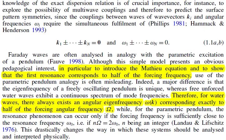
There are some clues to this idea in this recent ground-breaking article on sloshing wave modeling by Rajchenbach et al [1]. Their equation (1.1b) in the figure below suggests that three waves are needed to simultaneous fulfill the requirement of the frequencies summing to zero for multiwave coupling.

from Rajchenbach, Jean, and Didier Clamond. “Faraday waves: their dispersion relation, nature of bifurcation and wavenumber selection revisited.” Journal of Fluid Mechanics 777 (2015): R2. [1]

Adding a period of 83 years — which is often touted as the Gleissberg cycle [2] — to the (8.85, 18.6) pair will generate the quad set of (6.47, 14.0, 5.59, 21.2). These sum to zero as 1/6.47+1/14-1/5.59-1/21.2 ~ -0.00007. Intriguingly, the 5.59 period is a strong term in the ENSO model fit — note in the figure below the power spectrum peaks highlighted in yellow are the biennial-modulated set of these terms (ignore the x-axis label as that should be in units of 2048/months). On the other hand, the 21.2 year period is either weak or overfits with an existing 18.6 year term (centered peaks marked with a red dash). Seasonally aliased anomalistic periods are marked by blue dashes. Collectively these terms account for the vast majority of the power in the spectrum.

In the Rajchenbach article excerpt above, they note that period doubling is an emergent feature of nonlinear waves when modeled by the Mathieu equation. The nonlinearity comes from mutiplicative mixing of waves of different periods. Period doubling is somewhat reinforcing, as a harmonic that has a period of one year when mixed with a period of two years will recover the two year period.

But the “somewhat reinforcing” is a caveat, as what decides the alignment of the doubling on an odd versus even year is inherently arbitrary and therefore metastable.

An interesting wave sloshing behavior experiment somebody did — perhaps for a school project — apparently trying to duplicate the PRL paper “Observation of star-shaped surface gravity waves” by Rajchenbach et al (2013) is shown below. Watch closely and you can see that the 3-fold symmetry has a repeat cycle which is twice the period of the vertical forcing cycle. That is essentially a bifurcation leading to period doubling.

The odd symmetry of the wave sloshing shown may be classified as a tripole of sorts. One can almost see the potential tri-fold symmetry of the wave sloshing in this paper discussing a Pacific Ocean tripole.

from Henley, Benjamin J., et al. “A tripole index for the interdecadal Pacific oscillation.” Climate Dynamics 45.11-12 (2015): 3077-3090.

My own theory is that climate shifts such as occur with the IPO (circa late 1970’s) are associated with a period doubling phase inversion between even and odd years.

References

[1] J. Rajchenbach and D. Clamond, “Faraday waves: their dispersion relation, nature of bifurcation and wavenumber selection revisited,” Journal of Fluid Mechanics, vol. 777, p. R2, 2015. PDF here → rajchenbach2015

[2] One common estimate of the Gleissberg cycle is 83 years, but it is often referred to by a range of numbers. Several sources cite the 11.86 year Jupiter orbital period and the fact that it aligns with 83.02 years after 7 cycles. As this geometry will have a strong additive effect with the same seasonal date, there might be something to this — apart from Jupiter having a strong pull relative to the other planets, its persistence over a period of time may compensate for the stronger yet more transient pull of the moon. Robert Grumbine discusses planetary impacts here in the context of the Chandler Wobble. (Another bit of coincidental numerology is that 11.86 years is precisely 10 Chandler Wobble periods of 1.186 years = 433 days)