Overturning Impulse

The only earth science class I took in college was limnology.

Of course I was a casual student of freshwater activities before that time, but certain behaviors of lakes were hammered home by taking this class. For example, the idea behind seasonal lake overturning. The overturning occurs as a singular event at a particular time of the year (monomictic once per year and dimictic twice per year, see figure to the right).
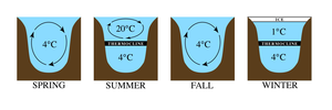
Saltwater doesn’t show the same predilection for overturning as freshwater does, mainly because of the higher density differences above and below the thermocline, but the thermocline does vary, especially at latitudes located off the equator.

The ENSO model that appears so promising might be pointing to a partial overturning  showing a bimictic behavior.  The bi-prefix implies a biennial impulse that reverses direction every year, tied into a biennial Mathieu modulation associated with fluid sloshing dynamics. The Mathieu modulation is partially induced from the forcing conditions [1][2].

The following figure shows the modulation and impulse forcing that generates the best fit for the ENSO model. The BLUE is the Mathieu modulation while the ORANGE is the impulse.

The impulse may be related to a rapidly changing slope when the bimictic partial-overturning kicks in. The positive impulse as the Mathieu modulation moves from high to low, and the negative impulse as the modulation moves from low to high, both occurring at the same relative time late in the year.  Note that the polarity of this may be reversed, as the lunar tidal forcing at the impulse time provides the strength of this forcing through a multiplicative effect. This is shown below.

Whether to call it sloshing or a partial overturning remains to be determined. Yet overall this piece of the puzzle is the primary ansatz behind the entire model — since if we don’t include it, the model does not generate the sharply distinct ENSO peaks and valleys. In other words, this is what causes the physical aliasing necessary to transform the monthly and fortnightly tidal cycles into a more erratic interannual cycling. This is in fact a simple model that shows more complex but still predictable dynamics.

References

[1] T. B. Benjamin and F. Ursell, “The stability of the plane free surface of a liquid in vertical periodic motion,” presented at the Proceedings of the Royal Society of London A: Mathematical, Physical and Engineering Sciences, 1954, vol. 225, pp. 505–515.

[2] S. Bale, K. Clavin, M. Sathe, A. S. Berrouk, F. C. Knopf, and K. Nandakumar, “Mixing in oscillating columns: Experimental and numerical studies,” Chemical Engineering Science, vol. 168, pp. 78–89, 2017.

ENSO forcing – Validation via LOD data

If we don’t have enough evidence that the forcing of ENSO is due to lunisolar cycles, this piece provides another independent validating analysis. What we will show is how well the forcing used in a model fit to an ENSO time series — that when isolated — agrees precisely with the forcing that generates the slight deviations in the earth’s rotational speed, i.e. the earth’s angular momentum. The latter as measured via precise measurements of the earth’s length of day (LOD).  The implication is that the gravitational forcing that causes slight variations in the earth’s rotation speed will also cause the sloshing in the Pacific ocean’s thermocline, leading to the cyclic ENSO behavior.

Continue reading →

ENSO and Fourier analysis

Much of tidal analysis has been performed by Fourier analysis, whereby one can straightforwardly deduce the frequency components arising from the various lunar and solar orbital factors. In a perfectly linear world with only two ideal sinusoidal cycles, we would see the Fourier amplitude spectra of Figure 1.

Fig 1: Amplitude spectra for a signal with two sinusoidal Fourier components. To establish the phase, both a real value and imaginary value is plotted.

Continue reading →

ENSO Proxy Validation

This is a straightforward validation of the ENSO model presented at last December’s AGU.

What I did was use the modern instrumental record of ENSO — the NINO34 data set — as a training interval, and then tested across the historical coral proxy record — the UEP data set.

The correlation coefficient in the out-of-band region of 1650 to 1880 is excellent, considering that only two RHS lunar periods (draconic and anomalistic month) are used for forcing. As a matter of fact, trying to get any kind of agreement with the UEP using an arbitrary set of sine waves is problematic as the time-series appears nearly chaotic and thus requires may Fourier components to fit. With the ENSO model in place, the alignment with the data is automatic. It predicts the strong El Nino in 1877-1878 and then nearly everything before that.

Continue reading →

ENSO and Tidal SLH – A Biennial Connection

[mathjax]It’s becoming abundantly clear that ENSO is driven by lunisolar mechanisms, especially true considering that we use the preferred models describing sloshing of water volumes — the Mathieu equation and the delay differential equation. What’s more, given the fact that the ENSO model works so well, one can guess that a connection between ENSO and lunar tidal forces should carry over to models for historical sea-level height (SLH) tidal data.

From my preliminary work analyzing SLH tidal data in 2014, I found an intriguing pattern relating to the same biennial pattern observed in the ENSO model. An extract from that post is reproduced below:

“The idea, related to delay differential equations, is to determine if it is at all possible to model at least part of ENSO (through the SOI) with data from a point in time in the tidal record with a compensated point from the past. This essentially models the effect of the current wave being cancelled partially by the reflection of a previous wave.

This is essentially suggesting that $$SOI = k f(t) – k f(t-Delta t)$$ where f(t) is the tidal record and k is a constant.

After some experimenting, a good fit is obtained when the current tidal data is set to 3 months ago, and the prior data is taken from 26 months in the past. To model the negative of ENSO, the 3-month old data is subtracted from the 26-month old data, Figure 1:”

Fig 1: Model of ENSO uses Tidal Gauge readings from Sydney Harbor.

This observation suggests a biennial pattern whereby high correlations in the time series occur for events observed close to two-years apart, with the difference taken up by the ENSO signal. The latter is at least partly due to the inverted barometer effect on SLH.

The sensitivity of the biennial effect is shown in the following contour diagram, where the peak CC is indicated and a slanted line showing the 2-year differencing points (table of the correlation coefficients here)

Focussing on the mechanisms for the correlation, the predictor can be reformulated as

f(t) = f(t-Delta t) + SOI / k


or that the 2-year prior SLH reading, with the addition of the SOI signal, will accurately represent the current SLH reading subject to a ~3 month lag.

My thinking is that this correlation can only occur if there is an actual biennial signal in the SLH itself. We can mathematically conjecture what is happening with the two year differencing by assuming that the SLH has the same height offset whenever pairs of points are separated by two years. You can see this in the following figure:

This brings up an interesting question as to why this biennial signal apparently can’t be detected via conventional means. A likely guess is because it gets obscured by the ENSO signal. And since the ENSO signal has never been adequately modeled, no one has an inkling that a biennial signal coexists in the mix. Yet this unconventional delay differencing approach (incidentally discovered with the help of machine learning) is able to discern it with a strong statistical significance.

The gist of this discovery is that a biennial tidal SLH motion exists and likely contributes (or at least identifies) the nonlinear biennial modulation driving the ENSO model described in previous posts.

Summary:

ENSO has elements of an annual teeter-totter. If you look through the research literature, you will find numerous references to a hypothesized behavior that one annual peak is followed by a lesser peak the next year. Yet, no evidence that this strict biennial cycle is evidence in the data — it’s more of a hand-wavy physical argument that this can or should occur.

The way to model this teeter-totter behavior is via Mathieu equations and delay differential equations. Both of these provide a kind of non-linear modulation that can sustain a biennial feedback mechanism.

The other ingredient is a forcing mechanism. The current literature appears to agree that this is due to prevailing wind bursts, which to me seems intuitive but doesn’t answer what forces the wind in the first place. As it turns out, only two parameters are needed to force the DiffEq and these align precisely with the primary lunar cycles that govern transverse and longitudinal directional momentum, the draconic and anomalistic months.

http://GeoEnergyMath.com/2017/05/01/the-enso-model-turns-into-a-metrology-tool/

Note the following table and how the draconic and anomalistic values zone in on the true value when correlating model against data:

Fitting the DiffEq values progressively away from the true value for the lunar tidal cycle results in a smaller correlation coefficient.

Having one of these values align may be coincidence, but having both combine with that kind of resolution is telling. The biennial connection to SLH tidal measurements is substantiation that a biennial modulation is intrinsic to the physical process.

Tidal Model of ENSO

The input forcing to the ENSO model includes combinations of the three major lunar months modulated by the seasonal solar cycle. This makes it conceptually similar to an ocean tidal analysis, but for ENSO we are more concerned about the long-period tides rather than the diurnal and semi-diurnal cycles used in conventional tidal analysis.

The three constituent lunar month factors are:

Month type Length in days
anomalistic 27.554549
tropical 27.321582
draconic 27.212220

So the essential cyclic terms are the following phased sinusoids

Continue reading →

Solution to Pulsed Mathieu Equation

Here is a bit of applied math that I have never seen described before.  It considers solving a variant of the Mathieu differential equation, an unwieldy beast that finds application in models of fluid sloshing (among others). Normally the Mathieu equation is only solvable as a stimulus forcing function convolved against the transcendental Mathieu function. Tools such as Mathematica include the Mathieu function in their library, but any other solution would require a full numerical DiffEq integration.

This is the typical Mathieu equation formulation:

f''(t) + ( omega_0^2 + B cos (nu_0 t) ) f(t) = 0


But instead of this nonlinear time-varying DiffEq, consider that we replace the sinusoidal modulation with a delta pulse. This is precisely our model of ENSO that we are trying to create from first principles. The pulse represents a forcing impulse from the alignment of a lunar and solar tidal cycle.

f''(t) + ( omega_0^2 + B delta (t) ) f(t) = 0


Taking the Laplace transform, we quickly arrive at what looks like an ordinary 2nd-order differential equation solution, albeit with an interesting initial condition:

s^2 F(s) + omega_0^2 F(s) + B f(0) = 0


After taking the inverse Laplace transform, we have:

f(t) = I(t) ast B f(0) delta(t)


where I(t) represents the impulse response of the first two terms, which is then convolved with a delta function evaluated at a value of f(t) for t=0. This is the only remnant of the nonlinear nature of the classical Mathieu function, in that the initial condition has a scaling proportional to the value of the function at that time. On the other hand, the solution to an ordinary DiffEq would not be dependent on the value of the function.

Thereafter we can extend this to a general solution; by creating a pulse train of delta functions we get this final convolution:

f(t) = I(t) ast B sum_{n=0}^{infty} f(t - n T) delta(t - n T)


where T is the pulse train period.

This is straightforward to evaluate for any pulse train — all we have to do is keep track of the changing value of f(t) as we come across each pulse.

Fig 1: A pulse train with both annual and biannual contributions.

In the above figure, why does the annual pulse have a two-year periodicity? That’s due to the alignment of a non-congruent tidal period with a seasonal pulse in terms of a Fourier series as described here and mathematically refined here.

If that is not intuitive, we can still consider it more of an anzat and see where it takes us.

For an ENSO time series, we an convolve the above delta pulse train with a set of known tidal periods of arbitrary amplitude and phase. For a fit trained up to 1980, this is the extrapolation post-1980:

Fig 2: Fit of pulsed Mathieu equation using a set of tidal periods as a forcing function. The impulse response here is a simple year-long rectangular window, i.e. the response has a memory of only a calendar year. This can be further refined if necessary. Yet, the projected time-series evaluated out-of-band from the fitting interval does a good job of capturing the ENSO profile.

The projected waveform matches the last 16 years very effectively considering how noisy the ENSO series is, and is very close to the fit over the entire interval. This is apart from the possible perturbation around the 1982 El Nino. The fact that the monthly tidal periods differ by slight amounts dictates that long multi-decadal intervals should be used for fitting. (In contrast, the model of QBO is primarily Draconic so the fitting interval can be much shorter)

Fig 3: Fit over the entire interval. The set of tidal periods applied was limited to the 3 major months (draconic, anomalistic, and sidereal/tropical) and the multiplicative combinations creating the fortnightly tides. This may not be enough to get the details right but erred on the side of under-fitting to establish the physical mechanism.

This approach is the logical follow-on to the wave transformed fitting approach that I had been using, most recently here and here. Both of these approaches are equally clever, which is a necessary ingredient when one is dealing with the unwieldy Mathieu equations. Moreover they both pull out the obvious stationary aspects of the ergodic ENSO time series.

The ENSO Challenge

It’s been quite a challenge decoding the physics of ENSO. Anything that makes the model more complex and with more degrees of freedom needs to be treated carefully. The period doubling bifurcation properties of wave sloshing has been an eye-opener for me. I experimented with adding a sub-harmonic period of 4 years to the 2-year Mathieu modulation and see if that improves the fit. By simply masking the odd behavior around 1981-1983, I came up with this breakdown of the RHS/LHS comparison.

Continue reading →

QBO Split Training

As with ENSO, we can train QBO on separate intervals and compare the fit on each interval.  The QBO 30 hPa data runs from 1953 to the present.  So we take a pair of intervals — one from 1953-1983 (i.e. lower) and one from 1983-2013 (i.e. higher) — and compare the two.

The primary forcing factor is the seasonally aliased nodal or Draconic tide which is shown in the upper left on the figure.  The lower interval fit in BLUE matches extremely well to the higher interval fit in RED, with a correlation coefficient above 0.8.

These two intervals have no inherent correlation other than what can be deduced from the physical behavior generating the time-series.  The other factors are the most common long-period tidal cycles, along with the seasonal factor.  All have good correlations — even the aliased anomalistic tide (lower left), which features a pair of closely separated harmonics, clearly shows strong phase coherence over the two intervals.

That’s what my AGU presentation was about — demonstrating how QBO and ENSO are simply derived from known geophysical forcing mechanisms applied to the fundamental mathematical geophysical fluid dynamics models. Anybody can reproduce the model fit with nothing more than an Excel spreadsheet and a Solver plugin.

Here are the PowerPoint slides from the presentation.


