ENSO, AMO, PDO and common-mode mechanisms

The basis of the ENSO model is the forcing derived from the long-period cyclic lunisolar gravitational pull of the moon and sun. There is some thought that ENSO shows teleconnections to other oceanic behaviors. The primary oceanic dipoles are ENSO and AMO for the Pacific and Atlantic. There is also the PDO for the mid-northern-latitude of the Pacific, which has a pattern distinct from ENSO. So the question is: Are these connected through interactions or do they possibly share a common-mode mechanism through the same lunisolar forcing mechanism?

Based on tidal behaviors, it is known that the gravitational pull varies geographically, so it would be understandable that ENSO, AMO, and PDO would demonstrate distinct time-series signatures. In checking this, you will find that the correlation coefficient between any two of these series is essentially zero, regardless of applied leads or lags. Yet the underlying component factors (the lunar Draconic, lunar Anomalistic, and solar modified terms) may potentially emerge with only slight variations in shape, with differences only in relative amplitude. This is straightforward to test by fitting the basic ENSO model to AMO and PDO by allowing the parameters to vary.

The following figure is the result of fitting the model to ENSO, AMO, and PDO and then comparing the constituent factors.

First, note that the same parametric model fits each of the time series arguably well. The Draconic factor underling both the ENSO and AMO model is almost perfectly aligned, indicated by the red starred graph, with excursions showing a CC above 0.99. All of the rest of the CC’s in fact are above 0.6.

The upshot of this analysis is two-fold. First to consider how difficult it is to fit any one of these time series to a minimal set of periodically-forced signals. Secondly that the underlying signals are not that different in character, only that the combination in terms of a Laplace’s tidal equation weighting are what couples them together via a common-mode mechanism. Thus, the teleconnection between these oceanic indices is likely an underlying common lunisolar tidal forcing, just as one would suspect from conventional tidal analysis.

An obvious clue from tidal data

One of the interesting traits of climate science is the way it gives away obvious clues. This recent paper by Iz

Iz, H Bâki. “The Effect of Regional Sea Level Atmospheric Pressure on Sea Level Variations at Globally Distributed Tide Gauge Stations with Long Records.” Journal of Geodetic Science 8, no. 1 (n.d.): 55–71.
shows such a breathtakingly obvious characteristic that it’s a wonder why everyone isn’t all over it.  The author seems to be understating the feature, which is essentially showing that for certain tidal records, the atmospheric pressure (recorded in the tidal measurement location) is pseudo-quantized to a set of specific values.  In other words, for a New York City tidal gauge station, there are 12 values of atmospheric pressure between 1000 and 1035 mb that are heavily favored over all other values.
One can see it in the raw data here where clear horizontal lines are apparent in the data points:

Raw data for NYC station  (Iz, H Bâki. “The Effect of Regional Sea Level Atmospheric Pressure on Sea Level Variations at Globally Distributed Tide Gauge Stations with Long Records.” Journal of Geodetic Science 8, no. 1 (n.d.): 55–71.)

and for the transformed data shown in the histogram below, where I believe the waviness in the lines is compensated by fitting to long-period tidal signal factors (such as 18.6 year, 9.3 year periods, etc).

Histogram for transformed data for NYC station  Iz, H Bâki. “The Effect of Regional Sea Level Atmospheric Pressure on Sea Level Variations at Globally Distributed Tide Gauge Stations with Long Records.” Journal of Geodetic Science 8, no. 1 (n.d.): 55–71.

The author isn’t calling it a quantization, and doesn’t really call attention to it with a specific name other than clustering, yet it is obvious from the raw data and even more from the histograms of the transformed data.

The first temptation is to attribute the pattern to a measurement artifact. These are monthly readings and there are 12 separate discrete values identified so that connection seems causal. The author says

“It was shown that random component of regional atmospheric pressure tends to cluster at monthly intervals. The clusters are likely to be caused by the intraannual seasonal atmospheric temperature changes, which may also act as random beats in generating sub-harmonics observed in sea level changes as another mechanism.”
Nearer the equator, the pattern is not readily evident. The fundamental connection between tidal value and atmospheric pressure is due to the inverse barometric effect
“At any fixed location, the sea level record is a function of time, involving periodic components as well as continuous random fluctuations. The periodic motion is mostly due to the gravitational effects of the sun-earth-moon system as well as because of solar radiation upon the atmosphere and the ocean as discussed before. Sometimes the random fluctuations are of meteorological origin and reflect the effect of ’weather’ upon the sea surface but reflect also the inverse barometric effect of atmospheric pressure at sea level.”
So the bottom-line impact is that the underlying tidal signal is viably measured even though it is at a monthly resolution and not the diurnal or semi-diurnal resolution typically associated with tides.
Why this effect is not as evident closer to the equator is rationalized by smaller annual amplification
“Stations closer to the equator are also exposed to yearly periodic variations but with smaller amplitudes. Large adjusted R2 values show that the models explain most of the variations in atmospheric pressure  observed at the sea level at the corresponding stations. For those stations closer to the equator, the amplitudes of the annual and semiannual changes are considerably smaller and overwhelmed by random excursions. Stations in Europe experience similar regional variations because of their proximities to each other”
So, for the Sydney Harbor tidal data the pattern is not observed

Sydney histogram does not show a clear delineated quantization

Whereas, I previously showed the clear impact of the ENSO signal on the Sydney tidal data after a specific transform in this post. The erratic ENSO signal (with a huge inverse barometric effect as measured via the SOI readings of atmospheric pressure) competes with the annual signal so that the monthly quantization is obscured. Yet, if the ENSO behavior is also connected to the tidal forcing at these long-period levels, there may be a tidal unification yet to be drawn from these clues.

The ENSO Forcing Potential – Cheaper, Faster, and Better

Following up on the last post on the ENSO forcing, this note elaborates on the math.  The tidal gravitational forcing function used follows an inverse power-law dependence, where a(t) is the anomalistic lunar distance and d(t) is the draconic or nodal perturbation to the distance.

F(t) propto frac{1}{(R_0 + a(t) + d(t))^2}'

Note the prime indicating that the forcing applied is the derivative of the conventional inverse squared Newtonian attraction. This generates an inverse cubic formulation corresponding to the consensus analysis describing a differential tidal force:

F(t) propto -frac{a'(t)+d'(t)}{(R_0 + a(t) + d(t))^3}

For a combination of monthly and fortnightly sinusoidal terms for a(t) and d(t) (suitably modified for nonlinear nodal and perigean corrections due to the synodic/tropical cycle)   the search routine rapidly converges to an optimal ENSO fit.  It does this more quickly than the harmonic analysis, which requires at least double the unknowns for the additional higher-order factors needed to capture the tidally forced response waveform. One of the keys is to collect the chain rule terms a'(t) and d'(t) in the numerator; without these, the necessary mixed terms which multiply the anomalistic and draconic signals do not emerge strongly.

As before, a strictly biennial modulation needs to be applied to this forcing to capture the measured ENSO dynamics — this is a period-doubling pattern observed in hydrodynamic systems with a strong fundamental (in this case annual) and is climatologically explained by a persistent year-to-year regenerative feedback in the SLP and SST anomalies.

Here is the model fit for training from 1880-1980, with the extrapolated test region post-1980 showing a good correlation.

The geophysics is now canonically formulated, providing (1) a simpler and more concise expression, leading to (2) a more efficient computational solution, (3) less possibility of over-fitting, and (4) ultimately generating a much better correlation. Alternatively, stated in modeling terms, the resultant information metric is improved by reducing the complexity and improving the correlation — the vaunted  cheaper, faster, and better solution. Or, in other words: get the physics right, and all else follows.


ENSO model for predicting El Nino and La Nina events

Applying the ENSO model to predict El Nino and La Nina events is automatic. There are no adjustable parameters apart from the calibrated tidal forcing amplitudes and phases used in the process of fitting over the training interval. Therefore the cross-validated interval from 1950 to present is untainted during the fitting process and so can be used as a completely independent and unbiased test.

Continue reading →

Millennium Prize Problem: Navier-Stokes

Watched the hokey movie Gifted on a plane ride. Turns out that the Millennium Prize for mathematically solving the Navier-Stokes problem plays into the plot.

I am interested in variations of the Navier–Stokes equations that describe hydrodynamical flow on the surface of a sphere.  The premise is that such a formulation can be used to perhaps model ENSO and QBO.

The so-called primitive equations are the starting point, as these create constraints for the volume geometry (i.e. vertical motion much smaller than horizontal motion and fluid layer depth small compared to Earth’s radius). From that, we go to Laplace’s tidal equations, which are a linearization of the primitive equations.

I give a solution here, which was originally motivated by QBO.

Of course the equations are under-determined, so the only hope I had of solving them is to provide this simplifying assumption:

{frac{partialzeta}{partialvarphi} = frac{partialzeta}{partial t}frac{partial t}{partialvarphi}}


If you don’t believe that this partial differential coupling of a latitudinal forcing to a tidal response occurs, then don’t go further. But if you do, then:


Solar Eclipse 2017 : What else?

The reason we can so accurately predict the solar eclipse of 2017 is because we have accurate knowledge of the moon’s orbit around the earth and the earth’s orbit around the sun.

Likewise, the reason that we could potentially understand the behavior of the El Nino Southern Oscillation (ENSO) is that we have knowledge of these same orbits. As we have shown and will report at this year’s American Geophysical Union (AGU) meeting, the cyclic gravitational pull of the moon (lower panel in Figure 1 below) interacting seasonally precisely controls the ENSO cycles (upper panel Figure 1).

Fig 1: Training interval 1880-1950 leads to extrapolated fit post-1950

Figure 2 is how sensitive the fit is to the precise value of the lunar cycle periods. Compare the best ft values to the known lunar values here. This is an example of the science of metrology.

Fig 2: Sensitivity to selection of lunar periods.

The implications of this research are far-ranging. Like knowing when a solar eclipse occurs helps engineers and scientists prepare power utilities and controlled climate experiments for the event, the same considerations apply to ENSO.  Every future El Nino-induced heat-wave or monsoon could conceivably be predicted in advance, giving nations and organizations time to prepare for accompanying droughts, flooding, and temperature extremes.

Follow @whut on Twitter:

//platform.twitter.com/widgets.js

ENSO Split Training for Cross-Validation

If we split the modern ENSO data into two training intervals — one from 1880 to 1950 and one from 1950 to 2016, we get roughly equal-length time series for model evaluation.

As Figure 1 shows, a forcing stimulus due to monthly-range LOD variations calibrated to the interval between 2000 to 2003 (lower panel) is used to train the ENSO model in the interval from 1880 to 1950. The extrapolated model fit in RED does a good job in capturing the ENSO data in the period beyond 1950.

Fig. 1: Training 1880 to 1950

Next, we reverse the training and verification fit, using the period from 1950 to 2016 as the training interval and then back extrapolating. Figure 2 shows this works about as well.

Fig. 2: Training interval 1950 to 2016

Continue reading →

Deterministic and Stochastic Applied Physics

Pierre-Simon Laplace was one of the first mathematicians who took an interest in problems of probability and determinism.  It’s surprising how much of the math and applied physics that Laplace developed gets used in day-to-day analysis. For example, while working on the ENSO and QBO analysis, I have invoked the following topics at some point:

  1. Laplace’s tidal equations
  2. Laplace’s equation
  3. Laplacian differential operator
  4. Laplace transform
  5. Difference equation
  6. Planetary and lunar orbital perturbations
  7. Probability methods and problems
    1. Inductive probability
    2. Bayesian analysis, e.g. the Sunrise problem
  8. Statistical methods and applications
    1. Central limit theorem
    2. Least squares
  9. Filling in holes of Newton’s differential calculus
  10. Others here

Apparently he did so much and was so comprehensive that in some of his longer treatises he often didn’t cite the work of others, making it difficult to pin down everything he was responsible for (evidently he did have character flaws).

In any case, I recall applying each of the above in working out some aspect of a problem. Missing was that Laplace didn’t invent Fourier analysis but the Laplace transform is close in approach and utility.

When Laplace did all this research, he must have possessed insight into what constituted deterministic processes:

We may regard the present state of the universe as the effect of its past and the cause of its future. An intellect which at a certain moment would know all forces that set nature in motion, and all positions of all items of which nature is composed, if this intellect were also vast enough to submit these data to analysis, it would embrace in a single formula the movements of the greatest bodies of the universe and those of the tiniest atom; for such an intellect nothing would be uncertain and the future just like the past would be present before its eyes.

— Pierre Simon Laplace,
A Philosophical Essay on Probabilities[wikipedia]
This is summed up as:

He also seemed to be a very applied mathematician, as per a quote I have used before  “Probability theory is nothing but common sense reduced to calculation.”  Really nothing the least bit esoteric about any of Laplace’s math, as it seemed always motivated by solving some physics problem or scientific observation. It appears that he wanted to explain all these astronomic and tidal problems in as simple a form as possible. Back then it may have been esoteric, but not today as his techniques have become part of the essential engineering toolbox. I have to wonder if Laplace were alive now whether he would agree that geophysical processes such as ENSO and QBO were equally as deterministic as the sun rising every morning or of the steady cyclic nature of the planetary and lunar orbits. And it wasn’t as if Laplace possessed confirmation bias that behaviors were immediately deterministic; as otherwise he wouldn’t have spent so much effort in devising the rules of probability and statistics that are still in use today, such as the central limit theorem and least squares.

Perhaps he would have glanced at the ENSO problem for a few moments, noticed that in no way that it was random, and then casually remarked with one his frequent idiomatic phrases:

“Il est aisé à voir que…”  … or ..  (“It is easy to see that…”).

It may have been so obvious that it wasn’t important to give the details at the moment, only to fill in the chain of reasoning later.  Much like the contextEarth model for QBO, deriving from Laplace’s tidal equations.

Where are the Laplace’s of today that are willing to push the basic math and physics of climate variability as far as it will take them? It has seemingly jumped from Laplace to Lorenz and then to chaotic uncertainty ala Tsonis or mystifying complexity ala Lindzen. Probably can do much better than to punt like that … on first down even !

Scaling El Nino

Recently, the rock climber Alex Honnold took a route up El Capitan without ropes.There’s no room to fail at that. I prefer a challenge that one can fail at, and then keep trying.  This is the ascent to conquering El Nino:

The Free-thought Route*

Χ  Base camp:  ENSO (El Nino/Southern Oscillation) is a sloshing behavior, mainly in the thermocline where the effective gravity makes it sensitive to angular momentum changes.
Χ  Faster forcing cycles reinforce against the yearly cycle, creating aliased periods. How?
Χ  Monthly lunar tidal cycles provide the aliased factors: Numbers match up perfectly.
① This aliasing also works for QBO, an atmospheric analog of ENSO.
Χ  A biennial meta-stability appears to be active. Cycles reinforce on alternating years.
Χ  The well-known Mathieu modulation used for sloshing simulations also shows a biennial character.
② Machine learning experiments help ferret out these patterns.
Χ  The delay differential equation formulation matches up with the biennial Mathieu modulation with a delay of one-year.  That’s the intuitive yearly see-saw that is often suggested to occur.
③  The Chandler wobble also shows a tidal forcing tendency, as does clearly the earth’s LOD (length-of-day) variations.
Χ  Integrating the DiffEq model provides a good fit, including long-term coral proxy records
Χ  Solving the Laplace tidal equation via a Sturm-Liouville expression along the equator helps explain details of QBO and ENSO
④  Close inspection of sea-level height (SLH) tidal records show evidence of both biennial and ENSO characteristics
Δ Summit: Final validation of the geophysics comparing ENSO forcing against LOD forcing.

Model fits to ENSO using a training interval

The route encountered several dead-ends with no toe-holds or hand-holds along the way (e.g. the slippery biennial phase reversal, the early attempts at applying Mathieu equation). In retrospect many of these excursions were misguided or overly complex, but eventually other observations pointed to the obvious route.

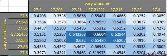
This is a magnification of the fitting contour around the best forcing period values for ENSO. These pair of peak values are each found to be less than a minute apart from the known values of the Draconic cycle (27.2122 days) and Anomalistic cycle (27.5545 days).

The forcing comes directly from the angular momentum variations in the Earth’s rotation. The comparison between what the ENSO model uses and what is measured via monitoring the length-of-day (LOD) is shown below:


*  This is not the precise route I took, but how I wish it was in hindsight.

Strictly Biennial Cycles in ENSO

Continuing from a previous post describing the historical evolution of ocean dynamics and tidal theory, this paper gives an early history of ENSO [1].

The El Niño–Southern Oscillation (ENSO) is among the most pervasive natural climate oscillations on earth, affecting the web of life from plankton to people. During mature El Niño (La Niña) events, the sea surface temperature (SST) in the eastern equatorial Pacific warms (cools), leading to global-scale responses in the terrestrial biosphere transmitted through modifications of large-scale atmospheric circulation. The dynamics of—and global responses to—ENSO have been studied for nearly eight decades (Walker and Bliss 1932; Ropelewski and Halpert 1989; Kiladis and Diaz 1989; Yulaeva and Wallace 1994). Cyclic patterns in climate events have also been connected to something resembling ENSO as early as the mid-nineteenth century. Reminiscing on his 1832 visit to Argentina during his expedition on the H.M.S. Beagle, British naturalist Charles Darwin notes “[t]hese droughts to a certain degree seem to be almost periodical; I was told the dates of several others, and the intervals were about fifteen years” (Darwin 1839). Nearly 60 years later, Darwin enters into his journal “. . . variations in climate sometimes appear to be the effect of the operation of some very general cause” (Darwin 1896). Some believe this “very general cause” was actually an early piecing together of ENSO and its now notorious impact on extreme weather events in South America (Cerveny 2005). It is only a coincidence that Darwin may have been among the first to point out the cyclic nature of ENSO, and the focus of this paper is the association between ENSO and the Galápagos Islands, which also owe their fame to Darwin.

Beyond this history, the purpose of this particular paper is to investigate the mechanics behind ENSO and to isolate the “very general cause” that Darwin first hypothesized (and isn’t it always the case how the most intellectually curious are at the root of scientific investigations?). According to this same paper[1], a “strictly biennial” cycle is routinely observed in ENSO when run with an ocean general circulation model (OGCM). Yet they observe correctly as quoted below that “Such strictly biennial regularity is not realistic, as ENSO in nature at present is neither perfectly regular nor significantly biennial.”

Note how strong the biennial Fourier factor is in their simulation (along with the perfectly acceptable harmonic at 2/3 year which will shape the biennial into anything from a triangle to a square wave). With our ENSO model, I can easily reproduce a strictly biennial cycle just by changing the forcing from a lunar monthly cycle (incongruent with a yearly cycle) to anything that is a harmonic with the yearly cycle. So it’s our claim that it’s the lunar cycle that remains the key factor that changes the ENSO cycle into something that is “neither perfectly regular nor significantly biennial” in the words of the cited paper. The biennial factor is still there but it gets modified and split by the lunar cycle to the extent that no biennial factor remains in the Fourier spectra.

Yet if we look into the GCM’s that researchers have developed and you will find that none have any capabilities for introducing a lunar tidal factor as a forcing.  Why is that?  Probably because someone long ago simply asserted that the lunar gravitational pull wasn’t important for ENSO, contrary to its critical importance for understanding ocean tides.   So is this lunar effect really the “very general cause” that Darwin was thinking of to explain ENSO?

As a result of some intellectual curiosity to actually test the tidal forcing against a biennial modulation, I think the answer is a definitive yes. This is how sensitive the fitting of the model is to selection of the two forcing cycles

By adjusting the values progressively away from the true value for the lunar tidal cycle (27.2122 days for the Draconic cycle and 27.55455 days for the Anomalistic cycle), it will result in a smaller correlation coefficient. This doesn’t happen by accident. Fitting this same model to 200 years of ENSO coral proxy data also doesn’t happen by accident. And extracting precisely phased and correlated lunar cycles to the actual forcing applied to the earth’s rotation also doesn’t happen by accident. I think it’s time for the GCM’s to revisit the role of lunar forcing, just as NASA JPL was about to before they decided to pull the plug on their own lunar research initiative [2].

References

[1] K. B. Karnauskas, R. Murtugudde, and A. J. Busalacchi, “The effect of the Galápagos Islands on ENSO in forced ocean and hybrid coupled models,” Journal of Physical Oceanography, vol. 38, no. 11, pp. 2519–2534, 2008.

[2]  From a post-mortem —  “None of the peer-reviewers nor collaborators in 2006 had anticipated that the most remarkable large-scale process that we were going to find comes from ocean circulations fueled by Luni-Geo-Solar gravitational energy.”