The input forcing to the ENSO model includes combinations of the three major lunar months modulated by the seasonal solar cycle. This makes it conceptually similar to an ocean tidal analysis, but for ENSO we are more concerned about the long-period tides rather than the diurnal and semi-diurnal cycles used in conventional tidal analysis.
The three constituent lunar month factors are:
| Month type | Length in days |
|---|---|
| anomalistic | 27.554549 |
| tropical | 27.321582 |
| draconic | 27.212220 |
So the essential cyclic terms are the following phased sinusoids


The draconic and tropical terms are combined because the tropical factor appears as a perturbation to the stronger draconic factor. As with QBO, the draconic tidal forcing is more of a global effect while the tropical forcing is isolated to a specific longitude for each nodal crossing.
The first two non-linear factors arise from the fortnightly contributions, which are essentially the squared terms for d(t) and a(t).
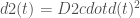

These terms d2(t) and a2(t) appear in tidal tables as low Doodson number periods of 13.606 days and 13.777 days respectively, shown below highlighted in yellow. The tropical term at 13.661 days is stronger (last column value), but that is for ocean tides, which acts as a more localized force than the wide-scale ENSO interaction.
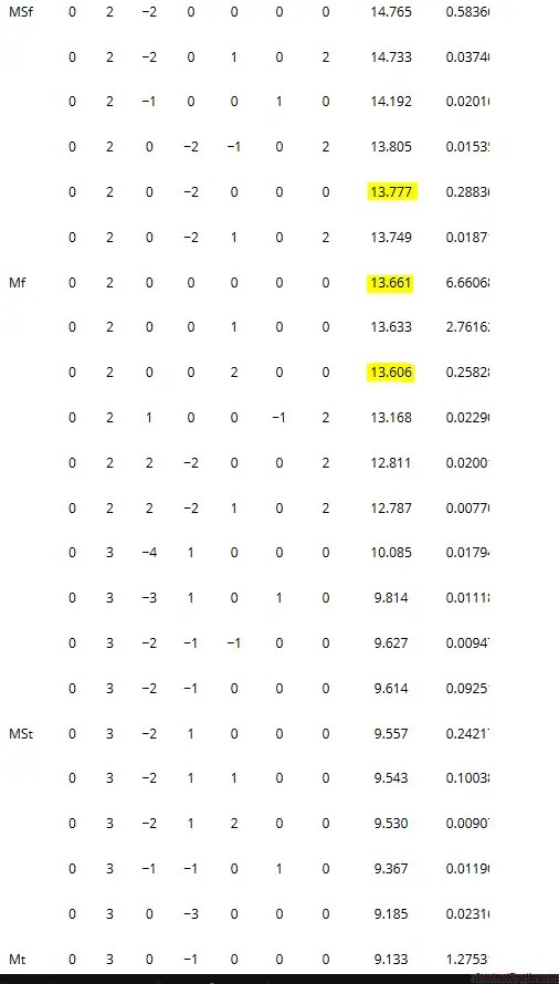
Fig 1 : Tidal table from “Long-period tidal variations in the length of day”, Ray and Erofeeva
Lastly, we have the non-linear cross-terms: da(t) a fortnightly term, two 9-day d2a(t) and da2(t), and a 6-day term d2a2(t).


So to first order, the forcing terms have only 3 phase factors :

and several amplitude factors :

All the other phase factors are set from the factor multiplications, with the phases retained from the base factors (d(t) and a(t)) . And those base phases are set from precise measurements of the nodal passage crossing dates (for d(t)) and the perigee and apogee dates (for a(t)). From those two sources, the sine phases for the Draconic and Anomalistic factors are -0.02 rads and -0.75 rads relative to an 1880 starting point. The phase is maintained over a long 100+ year interval dependent on the precision retained in the lunar tidal frequencies.
For the seasonal term, we introduce delta spikes at fixed points for each year or alternate year. This acts to impulse-modulate the tidal forcings such that the rapid lunar monthly cycles are singled out for amplification at specific times of the year. From Mathieu analysis, these spikes are found to occur in December of each year, alternating polarity for even and odd years, see Figure 2 below. This is essentially a 2 year sine wave with equal amplitude in each odd harmonic, as described here and here from a careful analysis of the aliased spectrum of tidal periods.
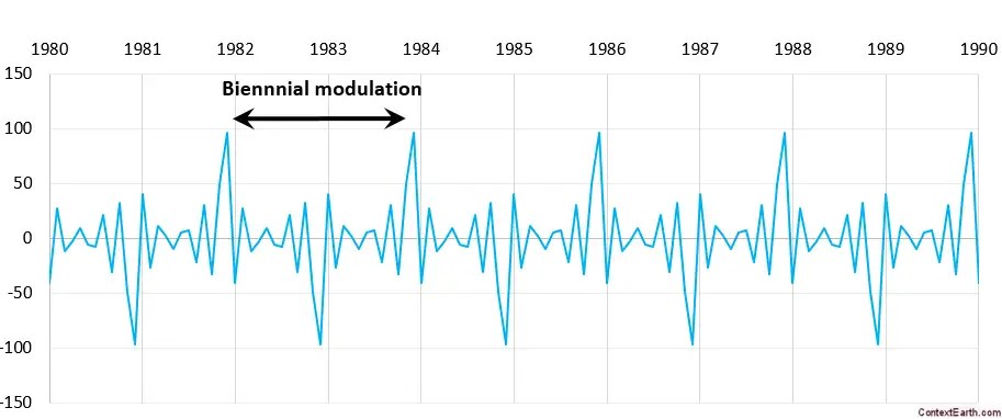
Fig 2: Seasonal impulse modulation applied to tidal forcing. this becomes the I(t) multiplicative factor in the model.
Going into even more detail, the ENSO model is able to discern the variation in the length (and phase) of the lunar Draconic month (see here https://eclipse.gsfc.nasa.gov/SEhelp/moonorbit.html#draconic) and in particular the Anomalistic month, which shows much greater variation. This is a detailed second-order effect that would only be possible to measure if the model of the first-order effect is correct.
Fig. 3 : Small variation in the Draconic month. This doesn’t provide a significant contribution to the model fit but appears to be detectable.
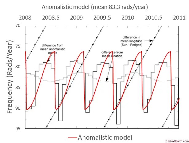
Fig 4 : Larger variation in the Anomalistic month. This precise alignment was found by the fitting procedure and appears to have significance in maintaining phase in the modeled periodic variation.
After taking all these factors into consideration, we formulate an expression combining the 8 amplitude forcing factors and then vary the amplitudes until we maximize the correlation coefficient correl(f,ENSO) over a fitting interval.
![f(t) = I(t) cdot [d(t) + a(t) + d2(t) + a2(t) + da(t) + d2a(t) + da2(t) + d2a2(t)]](https://s0.wp.com/latex.php?latex=f%28t%29+%3D+I%28t%29+cdot+%5Bd%28t%29+%2B+a%28t%29+%2B+d2%28t%29+%2B+a2%28t%29+%2B+da%28t%29+%2B+d2a%28t%29+%2B+da2%28t%29+%2B+d2a2%28t%29%5D+&bg=ffffff&fg=444444&s=0&c=20201002)
Since the forcing factors are spiked with a seasonal impulse I(t), we integrate over one year with a rectangular window as described in the previous post. This is not a Mathieu equation but a simpler forced response to a basic differential equation; thus providing a basic entry level analysis. It can all be done on an Excel spreadsheet with the Solver add-in.
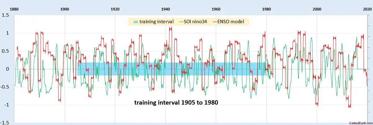
Fig 5 : Solver fit to ENSO model, with fixed tidal phases and varying amplitudes. The ENSO signal was compressed by taking a square root of the unsigned amplitude and then carrying over the original sign. There is good reason to assume that the velocity is the actual measure and not the velocity squared or kinetic energy = gravity head of the ENSO profile.
The correlation coefficient of the model fit to the data is higher over the last 25 years than it is within the training interval. So if we take this last 25 years and train on this interval, the past seems to back-project remarkably well also (see Figure 6 below).
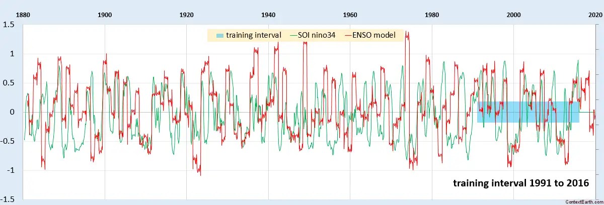
Fig 6 : Solver fit over a very short interval. Over-fitting doesn’t seem to have a deleterious impact as it typically would in such a short fitting interval because the phase relationships between the factors are highly constrained.
Even though this is a very crude analysis it seems to capture the behavior effectively via a straightforward mechanical fitting algorithm. The amount of over-fitting is actually quite constrained [1], as the phase factors and cascaded multiplications from the base terms don’t allow as many degrees of freedom as one would first imagine. One can do a similar fitting for QBO and this is actually more impressive as the Draconic term dominates the forcing, see Figure 7 below. I will discuss this more in a future post, as the contrast between ENSO and QBO is informative.
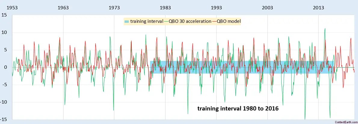
Fig 6: QBO fitting results using a similar approach as that used for the ENSO data
The strongest commonality between QBO and ENSO is the reliance on lunisolar forcing. We’ve slowly chipped away at the models of each until that salient factor emerges as the primary forcing driver. In particular, the Chandler wobble appears to be precisely temporally aligned with the seasonally reinforced Draconic lunar forcing, thus simplifying the my original interpretation substantially. Eliminating the noise from the ENSO data set is still an ongoing concern, as the fitting algorithm can’t discern the noise from the signal.
Update: Here is a spreadsheet of the model. To run the model fit, download and select the Solver plug-in from the Data menu.
Summary
The AGU-2016 ENSO model is turning out to be based entirely on the long-period lunar tidal cycles and the seasonal cycle. The same numerical techniques used for modeling ocean tides are applied, but with a different concept for seasonal reinforcing. The model therefore has gone from being an explanation of the ENSO behavior to a sensitive metrology technique — specifically for measuring lunar and solar cycles based on the sloshing sensitivity of a layered-fluid medium to forcing changes.
That’s one way you substantiate a model’s veracity — flip it from a question of over-fitting to one of precisely identifying physical constants. It’s not quite at the level of QBO but perhaps only a matter of time before a more refined model will demonstrate conclusively the deterministic aspects of ENSO. This will finally debunk the chaos proponents of ENSO including the AGW-denialists Judith Curry and Anastasios Tsonis. These two use the unpredictability of ENSO as leverage to push their anti-science political agenda claiming that any warming is obscured by random natural fluctuations.
Footnote
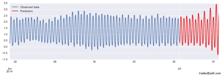
[1] See this tidal analysis for a potential example of overfitting. Too many sinusoidal terms are used in the fitting interval so that the extrapolated projection starts to diverge wildly to the right. That’s a characteristic of over-fitting — the over-fitted interval starts to diverge outside that interval as sinusoidal terms close in period start to constructively interfere and thus grow in strength.

Pingback: Shortest Training Fit for ENSO | context/Earth
Tried to post this over at ATTP’s, but WordPress really doesn’t like me 🙂
—————-
SM – I think you are overly optimistic that simply reviewing GCM code and making a few changes is all that’s needed.
How do we put tides in GCMs?
The accuracy of surface elevations in forward global barotropic and baroclinic tide models, Arbic et al, 2004, doi:10.1016/j.dsr2.2004.09.014 (PDF) lists 10 different parameters that need to be set. The anomalistic month appears as Mm, but geoenergymath/WHUT’s Tidal Model of ENSO also requires the tropical and draconic numbers.
The limitations, computational expense, and difficulty in achieving this is probably best spelled out by reading Concurrent simulation of the eddying general circulation and tides in a global ocean model, Arbic et al, 2010, https://doi.org/10.1016/j.ocemod.2010.01.007 (pre-print pdf).
BTW,at the required resolution and timestep necessary you end up generating lots and lots of data.
LikeLike
That’s cool, thanks. Mf is the fortnightly tropical tide which is half the 27.32 day value.
The distinction between Draconic and Tropical is that Tropical is more important as a local effect because it has a strong longitudinal component, while Draconic is a global effect due to the fact that it holds the nodal crossing period.
I have the same problem in commenting at ATTP, after trying for months. I finally decided to comment with a different wordpress account, and that seemed to do the trick. But now Willard thinks I am a sockpuppet.
LikeLike
Pingback: Reverse Engineering the Moon’s Orbit from ENSO Behavior | context/Earth