Useful to note that the majority of the posts written for this blog are in support of the mathematical analysis formulated in Mathematical Geoenergy (Wiley/AGU, 2018). As both new data becomes available and new techniques for model fitting & parameter estimation — aka inverse modeling (predominantly from the machine learning community) — are suggested, an iterative process of validation, fueled by the latest advancements, ensures that the GeoEnergyMath models remain robust and accurately reflective of the underlying observed behaviors. This of course should be done in conjunction with submitting significant findings to the research literature pipeline. However, as publication is pricey, my goal is to make the cross-validation so obvious that I can get an invitation for a review paper — with submission costs waived. Perhaps this post will be the deal-maker — certainly not the deal-breaker, but you can be the judge.
Continue readingForecasting
Full Wave Forcing
MSet
Global Models of Sea Surface Temperature
These are a set of 6 EOFs that describe the global SST in terms of a set of orthogonal time-series — essentially non-overlapping, each having a cross-correlation of ~0.0 with the others, like a sine/cosine pair, but in both spatial and temporal dimensions.
Continue readingNo Dice

The comic strip reinforces how poor El Nino forecasts have been in the past. Soon enough machine learning will reproduce the correlation to long-period tidal forcing, substantiated by extensive cross-validation. The interval between 1940 and 1950 was not touched by a hand of god (i.e. the fitting procedure).

The Power of Darwin
Using the LTE model on the NINO4 ENSO time-series, I excluded the interval between 1870-1875 for cross-validation. The fit below is from scratch on a dLOD-calibrated initial forcing, then allowing the values to vary slightly but the dLOD remains at 0.9999668 of the initial calibration.

The cross-validation doesn’t look good and actually is anti-correlated to a CC = -0.5 over that interval. But the region before 1875 appears suspiciously flat in any case, see the data on the KNMI site — it’s only a certainty that the El Nino peak at 1877-1878 is real and not estimated.
So, the next step is to take the fit to NINO4 and apply it to the Darwin (SOI) time-series, applying the same fitting interval from 1875-present. Immediately, it captures the 3 positive excursions in the interval 1870 to 1875. And then letting the fit proceed to a high CC, the result is shown below:

The resultant fit in the excluded cross-validation region reaches 0.58, thus reversing the anti-correlation and confirming that the NINO4 time-series data prior to 1875 is likely incorrect.
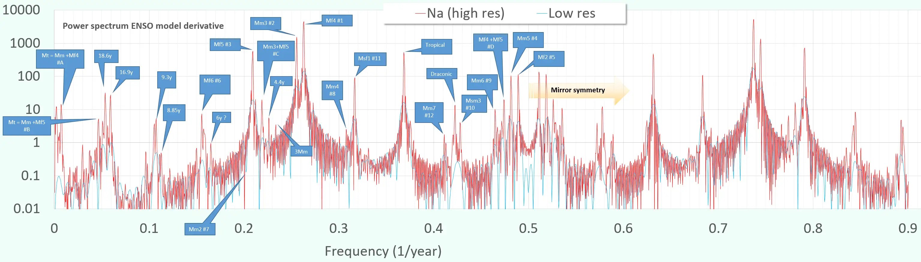
The fit data is at https://gist.github.com/pukpr/c26f1da00337e92dbb47671ca48af2cf?permalink_comment_id=4639783#gistcomment-4639783. The main modifications to tidal factors are in the very long periods — these values start small due to the dLOD calibration (the differential filters out low frequencies) but the 4.42 year amplitude is nearly tripled after the fit, the 8.85 & 9.3 year up by 50%. The 18.6 year is only up 14%, and the 3rd order 6 year and 15.9 year are down 63% and up 45% respectively. All the fortnightly and monthly values are stable. This is perhaps reasonable considering how much the LOD drifts over time at low frequency, and that the calibration is restricted to post-1962.
A Digital Twin of ENSO
The idea of a digital twin is relatively new in terms of coinage of terms, but the essential idea has been around for decades. In the past, a digital twin was referred to as a virtual simulation of a specific system, encoded via a programming language. In the case of a system that was previously built, the virtual simulation emulated all the behaviors and characteristics of that system, only operated on a computer, with any necessary interactive controls and displays provided on a console, either real or virtual. A widely known example of a VS is that of a flight simulator, which in historical terms was the industrial forerunner to today’s virtual reality. A virtual simulation could also be used during the design of the system, with the finished digital twin providing a blueprint for the actual synthesis of the end-product. This approach has also been practiced for decades, both in the electronics industry via logic synthesis of integrated circuits from a hardware description language and with physical products via 3D printing from CAD models.
Continue readingSub(Surface)Stack
I signed up for a SubStack account awhile ago and recently published two articles on this account (SubSurface) in the last week.
- https://pukite.substack.com/p/machine-learning-validates-the-enso
- https://pukite.substack.com/p/machine-learning-validates-the-amo
The SubStack authoring interface has good math equation mark-up, convenient graphics embedding, and an excellent footnoting system. On first pass, it only lacks control over font color.
The articles are focused on applying neural network cross-validation to ENSO and AMO modeling, as suggested previously. I haven’t completely explored the configuration space but one aspect that may becoming clear is the value of wavelet neural networks (WNN) for time-series analysis. The WNN approach seems much more amenable to extracting sinusoidal modulation of the input-to-output mapping — trained on a rather short interval and then cross-validated out-of-band. The Mexican hat wavelet (2nd derivative of a Gaussian) as an activation function in particular locks in quickly to an LTE modulation that took longer to find with the custom search software I have developed at GitHub. I think the reason for the efficiency is that it’s optimizing to a Taylor’s series expansion of the input terms, a classic nonlinear expansion that NN’s excel at.
The following training run using the Mexican hat activation and ADAM optimizer is an eye-opener, as it achieved an admirable fit within a minute of computation.

The GREEN on BLUE is training on NINO4 data over two end-point intervals, with the RED cross-validation over the out-of-band region. The correlation coefficient is 0.34, which is impressive considering the nature of the waveform. Clearly there is similarity.
Moreover, if we compare the model fit to data via the WNN against the LTE harmonics approach, you can also see where the two fare equally poorly. Below in the outer frame is the NINO4 LTE fit with the YELLOW arrow pointing downward at a discrepancy (a peak in the data not resolved in the fit). In comparison the yellow-bordered inset shows the same discrepancy on the WNN training run. So the fingerprints essentially match with no coaching.

The neural net chain is somewhat deep with 6 layers, but I think this is needed to expand to the higher-order terms in the Taylor’s series. In the directed graph below, L01 is the input tidal forcing and L02 is the time axis (with an initial very low weighting).

It also appears temporally stationary across the entire time-span, so that the WNN temporal contribution appears minimal.

In a previous fit the horizontal striations (indicating modulation factor at a forcing level) matched with the LTE model, providing further evidence that the the WNN was mapping to an optimal modulation.

The other Sub(Surface)Stack article is on the AMO, which also reveals promising results. This is a video of the training in action
Cross-validation
Cross-validation is essentially the ability to predict the characteristics of an unexplored region based on a model of an explored region. The explored region is often used as a training interval to test or validate model applicability on the unexplored interval. If some fraction of the expected characteristics appears in the unexplored region when the model is extrapolated to that interval, some degree of validation is granted to the model.
This is a powerful technique on its own as it is used frequently (and depended on) in machine learning models to eliminate poorly performing trials. But it gains even more importance when new data for validation will take years to collect. In particular, consider the arduous process of collecting fresh data for El Nino Southern Oscillation, which will take decades to generate sufficient statistical significance for validation.
So, what’s necessary in the short term is substantiation of a model’s potential validity. Nothing else will work as a substitute, as controlled experiments are not possible for domains as large as the Earth’s climate. Cross-validation remains the best bet.
Continue readingMf vs Mm
In an earlier post, the observation was that ENSO models may not be unique due to the numerous possibilities provided by nonlinear math. This was supported by the fact that a tidal forcing model based on the Mf (13.66 day) tidal factor worked equally as well as a Mm (27.55 day) factor. This was not surprising considering that the aliasing against an annual impulse gave a similar repeat cycle — 3.8 years versus 3.9 years. But I have also observed that mixing the two in a linear fashion did not improve the fit much at all, as the difference created a long interference cycle which isn’t observed in the ENSO time series data. But then thinking in terms of the nonlinear modulation required, it may be that the two factors can be combined after the LTE solution is applied.
Continue readingLow #DOF ENSO Model
Given two models of a physical behavior, the “better” model has the highest correlation (or lowest error) to the data and the lowest number of degrees of freedom (#DOF) in terms of tunable parameters. This ratio CC/#DOF of correlation coefficient over DOF is routinely used in automated symbolic regression algorithms and for scoring of online programming contests. A balance between a good error metric and a low complexity score is often referred to as a Pareto frontier.
So for modeling ENSO, the challenge is to fit the quasi-periodic NINO34 time-series with a minimal number of tunable parameters. For a 140 year fitting interval (1880-1920), a naive Fourier series fit could easily take 50-100 sine waves of varying frequencies, amplitudes, and phase to match a low-pass filtered version of the data (any high-frequency components may take many more). However that is horribly complex model and obviously prone to over-fitting. Obviously we need to apply some physics to reduce the #DOF.
Since we know that ENSO is essentially a model of equatorial fluid dynamics in response to a tidal forcing, all that is needed is the gravitational potential along the equator. The paper by Na [1] has software for computing the orbital dynamics of the moon (i.e. lunar ephemerides) and a 1st-order approximation for tidal potential:

The software contains well over 100 sinusoidal terms (each consisting of amplitude, frequency, and phase) to internally model the lunar orbit precisely. Thus, that many DOF are removed, with a corresponding huge reduction in complexity score for any reasonable fit. So instead of a huge set of factors to manipulate (as with many detailed harmonic tidal analyses), what one is given is a range (r = R) and a declination ( ψ=delta) time-series. These are combined in a manner following the figure from Na shown above, essentially adjusting the amplitudes of R and delta while introducing an additional tangential or tractional projection of delta (sin instead of cos). The latter is important as described in NOAA’s tide producing forces page.

Although I roughly calibrated this earlier [2] via NASA’s HORIZONS ephemerides page (input parameters shown on the right), the Na software allows better flexibility in use. The two calculations essentially give identical outputs and independent verification that the numbers are as expected.
As this post is already getting too long, this is the result of doing a Laplace’s Tidal Equation fit (adding a few more DOF), demonstrating that the limited #DOF prevents over-fitting on a short training interval while cross-validating outside of this band.

or this

This low complexity and high accuracy solution would win ANY competition, including the competition for best seasonal prediction with a measly prize of 15,000 Swiss francs [3]. A good ENSO model is worth billions of $$ given the amount it will save in agricultural planning and its potential for mitigation of human suffering in predicting the timing of climate extremes.
REFERENCES
[1] Na, S.-H. Chapter 19 – Prediction of Earth tide. in Basics of Computational Geophysics (eds. Samui, P., Dixon, B. & Tien Bui, D.) 351–372 (Elsevier, 2021). doi:10.1016/B978-0-12-820513-6.00022-9.
[2] Pukite, P.R. et al “Ephemeris calibration of Laplace’s tidal equation model for ENSO” AGU Fall Meeting, 2018. doi:10.1002/essoar.10500568.1
[3] 1 CHF ~ $1 so 15K = chump change.