Cross-validation is essentially the ability to predict the characteristics of an unexplored region based on a model of an explored region. The explored region is often used as a training interval to test or validate model applicability on the unexplored interval. If some fraction of the expected characteristics appears in the unexplored region when the model is extrapolated to that interval, some degree of validation is granted to the model.

This is a powerful technique on its own as it is used frequently (and depended on) in machine learning models to eliminate poorly performing trials. But it gains even more importance when new data for validation will take years to collect. In particular, consider the arduous process of collecting fresh data for El Nino Southern Oscillation, which will take decades to generate sufficient statistical significance for validation.

So, what’s necessary in the short term is substantiation of a model’s potential validity. Nothing else will work as a substitute, as controlled experiments are not possible for domains as large as the Earth’s climate. Cross-validation remains the best bet.

As a practical aside, CV is not for the faint-of-heart, since anyone doing cross-validation will get accused of cheating (what they apparently refer to as researcher Degrees Of Freedom). Well, of course the “unexplored” data is there for anyone to see, so everyone is in the same boat when it comes to avoiding tainting the results or priming the pump, so to speak. Yet, this paranoia is strong enough that critics may use the rDOF excuse to completely ignore cross-validation results (see link above for example of me trying to get any interest in cross-validation of a Chandler wobble model — taint goes both ways apparently, in this case as prejudice i.e. biased pre-judging as to the modeler’s intent).

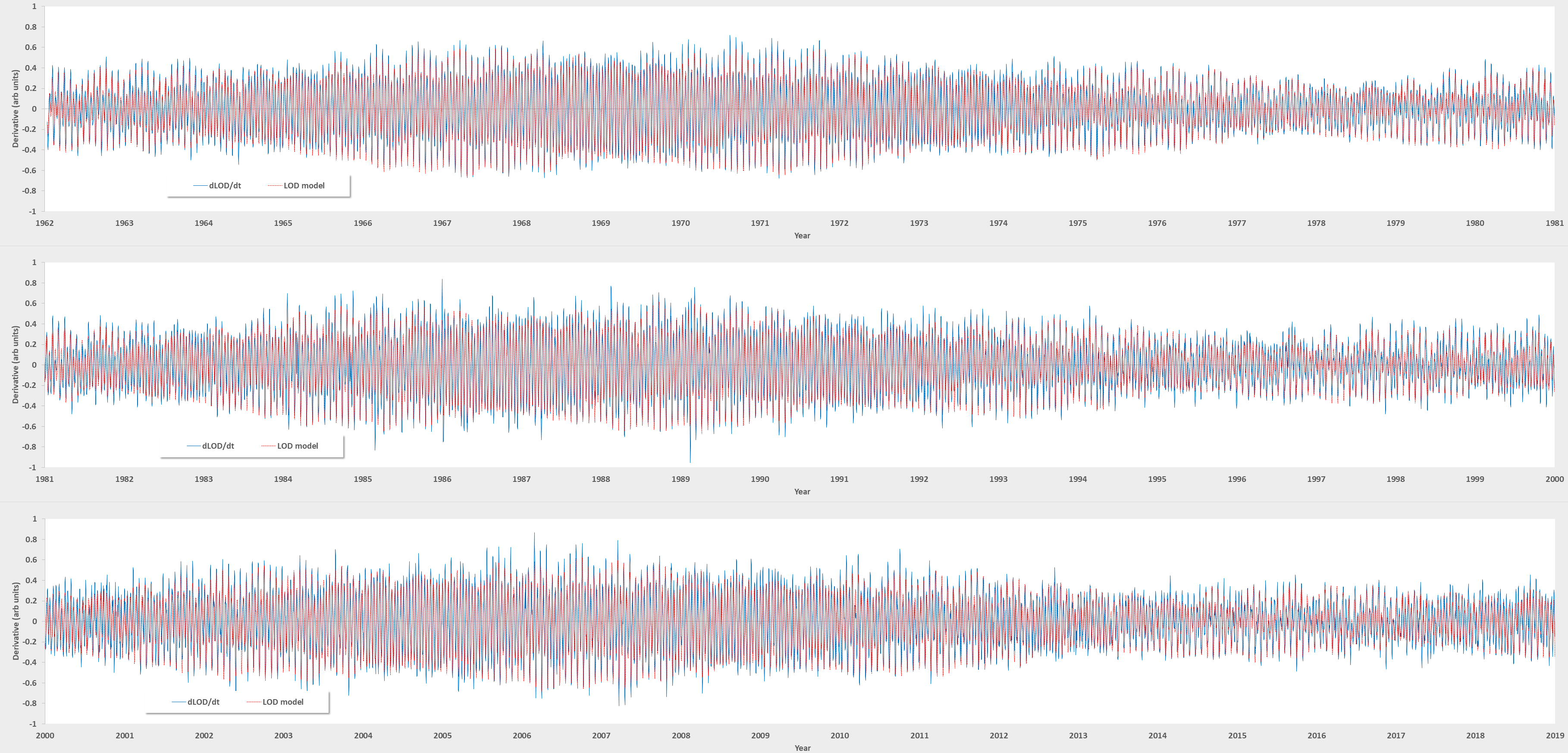
An effective yet non-controversial example is cross-validation of a delta Length-of-Day (dLOD) model. The LOD data is from Paris IERS and is transformed into an acceleration by taking the differential, thus dLOD. A cross-validation can easily be generated by taking any interval in the time series, fitting that to an appropriate model of the geophysics, and then extrapolating over the rest of the length (which stretches from 1962 to the current day). To do that, first we need to select the physical factors that will act to modify the angular momentum of the Earth’s rotation — these factors are simply the tidal torques as generated by the moon and sun, tabulated by R.D. Ray in “Long-period tidal variations in the length of day” (see Table 3, column labeled V₀/g for forcing values, with amplitude scaled by frequency since this is a differential LOD).

The strongest 30 tidal factors are arranged as a Fourier series and then optimally fit using a maximum linear regression algorithm (source code). The results (raw fit here) are shown below for 3 orthogonal training intervals, each approximately 20 years each (1962-1980, 1980-2000, and 2000-present).

It appears that Ray may have evaluated his predicted forcing values against similar LOD data, as the cross-validation agreement is very good across the board. He writes:

“The only realistic test of this new tidal LOD model is to examine how well it removes tidal energy from real LOD measurements. To test that we use the SPACE2008 time series of Earth rotation variations produced by Ratcliff and Gross [2010] from various types of space-geodetic measurements. Their method employs a specially designed Kalman filter to combine disparate types of measurements and to produce a time series with daily sampling interval; see also Gross et al. [1998]. After computing and subtracting the new LOD tidal model from the SPACE2008 data, we examine the residual spectrum for the possible presence of peaks at known tidal frequencies.”

This is an excellent example of effective cross-validation as the model is essentially stationary across the entire interval, indicating that the tidal factors represent the actual torque controlling the fastest cycling in the Earth’s LOD. Yes, it is possible that Ray applied his “researcher degrees of freedom” to further calibrate his tabulated tidal factors against this data, but it doesn’t detract from the excellent stationarity of the model itself. So as with a conventional tidal analysis, it doesn’t matter if a tidal model is calibrated via historical data cross-validation or from future data, as the foundational model has withstood the test of time as well as being internally self-consistent.

With that as a blueprint, we now enter the realm of non-linear model fitting a la ENSO. The relevant steps are reviewed in a recent blog post, which starts from the same set of tidal factors calibrated from dLOD data as described above. Keep in mind that allowing a researcher at least a few degrees of freedom to experiment with is the same as allowing them insight and educated guesses. Research would never advance without allowing flexibility when treading into unknown waters. So, the insight is to seed the initial model fitting with a few nonlinear modulation factors that represent the possible standing-wave modes of ENSO — one low-frequency modulation, and a high-frequency modulation set as a 7 & 14x harmonic of the fundamental, representing Tropical Instability Waves. The result of fitting the LTE model (using the GEM software) is shown below with the excluded-from-training intervals shown. Since these intervals were considered pristine from the point of view of the randomly mutating fitting process, any correlation between the model and the data within these intervals should be considered significant.

Click on the image’s link to magnify and get a sense on how well the model works in the highlighted validation intervals. There are essentially the 3 standing wave nodes (lower left), and the dLOD starting tidal factors (upper right) that are gradually varied to arrive at the final fit. It’s not perfect, but enough of the peaks and valleys align that not much additionally fitting is needed to model the data with a high correlation-coefficient across the entire time-series. As an example, including the pre-1880 ENSO data (which is somewhat iffy apart from the late-1870’s El Nino peak) generates this fit:

This “from scratch” cross-validation differs from the alternate approach of fitting to the entire interval and then excluding a portion before refitting, which is more suspect to bias (even though it can also show the effects of over-fitting as demonstrated in this experiment).

The difficulty in this scratch process, in contrast to the properties of the underlying dLOD model, is that the non-linear transformation required of LTE is much more structurally sensitive than the linear transformation of pure harmonic tidal analysis. For example, harmonic tidal analysis is essentially:

• f(t) = k F(t), where F(t) represents a set of tidal factors

so changes in k or F(t) reflect as a linear scaling in the output of f(t).

Whereas with the non-linear LTE model

• f(t) = sin(k F(t))

so that changes in k or F(t) can cause f(t) to swing wildly in both positive and negative direction.

The bottom-line is that the cross-validation results can’t be denied, but other researchers need to be involved in the process to improve the model enough to make it production quality. The LTE fitting software on GitHub is fast (it takes just a few minutes for the model to start aligning) and with a faster multi-CPU core (say try a 128 core) it would appeal to the scientific computing enthusiasts. As I designed the software to use all cores available, the speed-up would be nearly linear with number of cores. Could be down to minutes for a full fit, and thus very amenable to rapid turnaround experimentation.