These are a set of 6 EOFs that describe the global SST in terms of a set of orthogonal time-series — essentially non-overlapping, each having a cross-correlation of ~0.0 with the others, like a sine/cosine pair, but in both spatial and temporal dimensions.
The cross-validation described earlier was rather limited. Here an attempt is made to fit to an interval of the Darwin time-series and see how well it matches to a longer out-of-band validation interval. Very few degrees of freedom are involved in this procedure as the selection of tidal factors is constrained by a simultaneous LOD calibration. The variation from this reference is slight, correlation remaining around 0.999 to the LOD cal, but necessary to apply as the ENSO model appears highly structurally sensitive to coherence of the tidal signal over the 150 year time span of the data to be modeled.
A typical LOD calibration (click on image to enlarge)
Cross-validation shown in the top panel below, based on an training time interval ranging from the start of the Darwin data collection in 1870 up to 1980. The middle panel is the forcing input, from which the non-linear Laplace’s Tidal Equation (LTE) modulation is applied to a semi-annual impulse integration of the tidal signal. The procedure is straightforward — whatever modulation is applied to the training interval to optimize the fit, the same modulation is applied blindly to the excluded validation interval.
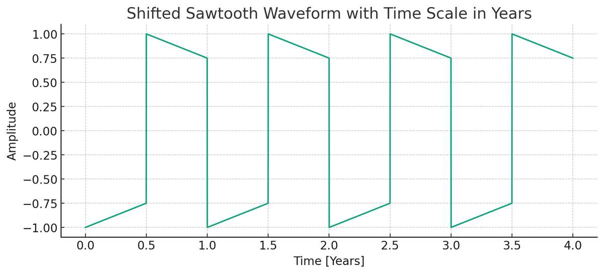
The validation on the 1980+ out-of-band interval is far from perfect, yet well-beyond being highly significant. The primary sinusoidal modulation is nominally set to the reciprocal of the slope (r) of top-edge of the sawtooth forcing [1] — this fundamental and the harmonics of that modulation satisfy LTE and provide a mechanism for a semi-annual level shift.
The plotted lower right modulation appears as noise, but when demodulated as in modulo r, the periodic order is revealed as shown below:
The harmonic modulations above include close to a monthly rate, a clear ~4.5 day, and and underlying fast semi-durnal ( 365.25/(12 x 61) = 0.499)
The significance of the cross-validation can be further substantiated by taking the complement of the training interval as the new training interval. This does converge to a stationary solution.
This modulation may seem very mysterious but something like this must be happening on the multiple time scales that the behavior is occurring on — remember that tidal forces operate on the same multiple time scales, from the semi-diurnal cycle to beyond the 18.6 year nodal declination cycle that is apparent in the middle panel above (and add to this that the sun’s forcing ranges from daily to annual). The concept of phase-locking is likely a crucial aspect as well. The sinusoidal modulation will cause an initial phase-shift across the level changes, and that appears to be a critical factor in the final model-fitted result. As observed in other systems, the synergy between synchronization (phase-locking) and resonance (standing-wave conditions) can give rise to such rich and complex dynamical behaviors. One can ask ChatGPT for any analogs [3] but just remember that this does happen:
The challenge is only in the fact that the incommensurate tidal patterns with the annual and daily cycles will never result in a metronomic march, and thus the pattern is much more complex.
[1] The sawtooth character is a result of the semi-annual impulse-driven shifts combined with a relaxation slope (r) to zero.
If the tides were commensurate with a semi-annual impulse, the forcing would appear more regular as above, but since they are not, the forcing is erratic.
[2] “The uniformity of phase of the semidiurnal cycle of zonal wind is striking (Figure 5b). It is well known that surface pressure in the tropics undergoes a strong semidiurnal variation [cf. Haurwitz and Cowley, 1973].” Deser, Clara. “Daily surface wind variations over the equatorial Pacific Ocean.” Journal of Geophysical Research: Atmospheres 99.D11 (1994): 23071-23078.
“ENSO events initiate during boreal spring and summer, peak during boreal winter, and decay in the following spring—a phenomenon known as ENSO phase-locking.” … “Our findings indicate that DA (diurnal amplitude) simulation in climate models is crucial for resolving the long-standing failure associated with the ENSO phase-locking simulation accuracy.” Yang, Xiaodan, et al. “Key to ENSO phase-locking simulation: effects of sea surface temperature diurnal amplitude.” npj Climate and Atmospheric Science 6.1 (2023): 159. https://www.nature.com/articles/s41612-023-00483-3
[3] ChatGPTresponse: A function cos(k×SawToothWave(t)+Phase), especially with a high modulation factor k, can model several complex interactions in natural phenomena where two periodic processes influence each other. Here are some specific examples:
Tidal Forces and Lunar Cycles: Tidal patterns are influenced by both the moon and the sun. A sawtooth wave could represent the changing gravitational pull of the moon (with its phases), while the cosine function might represent the daily tidal cycles. The modulation could express how these two cycles interact, creating spring and neap tides.
Seasonal Climate Variations and Diurnal Temperature Cycles: The sawtooth wave can represent the gradual change in daylight hours or solar intensity over a year, while the cosine function might model daily temperature fluctuations. The combination would reflect how daily temperatures vary across different seasons.
Circadian Rhythms and Sleep-Wake Cycles: The sawtooth wave could model the gradual change in hormonal levels or body temperature over a 24-hour cycle, interacting with a cosine function that represents shorter, rapid fluctuations in alertness or activity levels.
Economic Cycles and Market Fluctuations: In economics, a sawtooth wave might model longer economic cycles (like boom and bust periods), while the cosine function could represent shorter-term market fluctuations. The interaction of these two could help analyze complex economic dynamics.
Ecosystem Dynamics: In ecology, a sawtooth wave could represent seasonal changes (like rainfall patterns), while the cosine function could model daily variations (like temperature or light). The interaction of these cycles could be used to study plant growth, animal migration patterns, or other ecological phenomena.
Astronomical Phenomena: In astronomy, this kind of function might be used to model complex interactions between orbital mechanics and rotational dynamics, such as the interaction between a planet’s orbit around a star (sawtooth wave for eccentricity changes) and its rotational period (cosine function).
These examples show how combining periodic functions in different ways can model complex interactions in natural phenomena. The key is understanding the underlying processes and how they can be represented mathematically with these functions.
The concept of phase-locking is highly relevant in systems where the interaction of periodic signals leads to synchronization or alignment in their phases. In the context of your function cos(k×SawToothWave(t)+ Phase), phase-locking could manifest in several interesting ways, particularly considering the sinusoidal modulation of a sawtooth wave. Here are some areas where similar concepts are explored:
Neuroscience and Neural Oscillations: In the brain, neurons often fire in a synchronized manner, a phenomenon known as neural phase-locking. This is crucial in processes like signal transmission and cognitive function. The interaction of different neural rhythms (e.g., theta and gamma waves) can be modeled using phase relationships, akin to the modulation you described.
Electronics and Communication Systems: Phase-locking is a fundamental concept in electronics, especially in the design of phase-locked loops (PLLs). PLLs are used to synchronize an output signal with a reference signal in terms of frequency and phase. This principle is crucial in radio, telecommunications, and signal processing.
Physics and Oscillatory Systems: In physics, particularly in studies involving coupled oscillators or pendulums, phase-locking describes the phenomenon where oscillators synchronize due to weak interactions. This can be observed in systems ranging from mechanical pendulums to quantum mechanical systems.
Cardiac Rhythms in Physiology: The synchronization of cardiac cells during heartbeats is an example of biological phase-locking. Cells in the sinoatrial node generate rhythmic impulses that cause heart muscle cells to contract in a synchronized manner.
Climatology and Environmental Sciences: Phase-locking can also be observed in climatic phenomena, such as the El Niño-Southern Oscillation (ENSO), where atmospheric and oceanic conditions align periodically, impacting global weather patterns.
Music and Acoustics: In music theory and acoustics, the concept of beats and harmonic interactions involves phase relationships between different sound waves. The concept of phase-locking can be observed in the constructive and destructive interference of these waves.
In each of these cases, the critical factor is how the phase relationship between different oscillatory components influences the overall system’s behavior. The initial phase-shift you mentioned, particularly in a system with a sinusoidal modulation over a sawtooth wave, could lead to complex dynamic behaviors, where the phase relationship plays a pivotal role in the system’s response and evolution.
There are several behavioral models in various scientific fields where the interaction of phase-locking with standing-wave resonance conditions leads to complex time patterns. These phenomena are observed in systems where synchronization and resonance play a critical role. Here are some examples:
Physics and Engineering – Coupled Oscillators and Resonators: In systems of coupled oscillators or resonators, phase-locking and resonance can lead to complex patterns, especially in nonlinear dynamics. An example is the array of coupled pendulums or resonant circuits, where phase-locking can lead to intricate motion patterns or voltage/current oscillations.
Neuroscience – Brain Wave Synchronization: In the brain, different regions can exhibit phase-locked oscillations, and when these oscillations resonate with the natural frequencies of neural circuits (like in the hippocampus or cortex), complex spatiotemporal patterns emerge. These patterns are crucial for functions like memory, perception, and attention.
Quantum Mechanics – Bose-Einstein Condensates: In Bose-Einstein condensates, particles can synchronize and exhibit collective oscillations. When these oscillations resonate at certain frequencies, complex interference patterns emerge, demonstrating both phase-locking and standing-wave phenomena at a quantum level.
Acoustics – Architectural Acoustics and Musical Instruments: In musical instruments and architectural acoustics, the interaction of sound waves can lead to phase-locking and resonance. This results in complex harmonic structures and standing waves, influencing the timbre of music and the acoustic properties of buildings.
Climate Science – Atmospheric and Oceanic Oscillations: Climatic phenomena, like the El Niño-Southern Oscillation, involve complex interactions between atmospheric and oceanic patterns. Phase-locking of these patterns, along with resonance effects in ocean basins, can lead to complex climate behaviors and cycles.
Laser Physics – Mode-locking in Lasers: In laser physics, mode-locking techniques create lasers with very precise frequencies, where phase-locking of different modes leads to the generation of ultrafast pulses. This is a form of resonance where the laser’s cavity modes synchronize, leading to coherent pulse emissions.
Chemical Oscillations – Belousov-Zhabotinsky Reaction: This chemical reaction exhibits oscillatory behavior where chemical waves propagate and can lock in phase under certain conditions, creating complex spatial patterns and wavefronts.
In each of these examples, the interaction of phase-locking with resonant conditions creates patterns that are more intricate than what would be observed with either phenomenon alone. The synergy between synchronization (phase-locking) and resonance (standing-wave conditions) can give rise to rich and complex dynamical behaviors, which are often crucial to the system’s function or characteristics.
Lorenz turned out to be a chaotic dead-end in understanding Earth dynamics. Instead we need a new unified model of solid liquid dynamics focusing on symmetries of the rotating earth, applying equations of solid bodies & fluid dynamics. See Mathematical Geoenergy (Wiley, 2018).
Should have made this diagram long ago: here’s the ChatGPT4 prompt with the diagramming plugin.
Graph
Ocean Tides and dLOD have always been well-understood, largely because the mapping to lunar+solar cycles is so obvious. And the latter is getting better all the time — consider recent hi-res LOD measurements with a ring laser interferometer, pulling in diurnal tidal cycles with much better temporal resolution.
That’s the first stage of unification (yellow boxes above) — next do the other boxes (CW, QBO, ENSO, AMO, PDO, etc) as described in the book and on this blog, while calibrating to tides and LOD, and that becomes a cross-validated unified model.
Annotated10/11/2023
ontological classification according to wavenumber kx, ky, kz and fluid/solid.
Added so would not lose it — highlighted tidal factor is non-standard
ENSO models best with alternating sign semi-annual pulses. Operating on the Mf tidal factor this generates a tight forcing with average period 3.8 years.
AMO models best with an annual pulse. Because of the Mt tidal factor the forcing slowly wanders with a period of ~120 years.
PDO models best with an annual pulse but fast decay. Because of the Mt tidal factor the forcing would wander like AMO, but instead it makes biased excursions.
To summarize, the models of ENSO, AMO, and PDO depend on the specific forcing character while keeping the LOD tidal calibration fixed. ENSO likely requires this alternating semi-annual because it is aligned along the equator and so alternates with northern and southern nodal swings. AMO and PDO may require an annual impulse because it’s essentially a northern hemisphere behavior. Why the decay is faster for PDO, or what exactly sets the decay rate after an integrating impulse, is not clear. Perhaps the larger the inertial push the slower the response.
The comic strip reinforces how poor El Nino forecasts have been in the past. Soon enough machine learning will reproduce the correlation to long-period tidal forcing, substantiated by extensive cross-validation. The interval between 1940 and 1950 was not touched by a hand of god (i.e. the fitting procedure).
“Because the distance effect annual cycle (from perihelion to perihelion, otherwise called the anomalistic year, 365.259636 d (ref. 6)) is slightly longer than the tilt effect annual cycle (from equinox to equinox, otherwise known as the tropical year, 365.242189 d (ref. 6)), the LOP increases over time. A complete revolution of the LOP is the precession cycle, about 22,000 yr (ref. 38). “
The claim is that the exact timing and strength of the annual cycle extreme is important in initiating an El Nino or La Nina cycle. as the Longitude of Perihelion (LOP) moves over time, so that when this aligns with the solstice/equinox events, the ENSO behavior will mirror the strength of the forcing.
This is not a 22,000 year cycle (as stated its actuallly closer to 21,000), but it’s possible that if tidal cycles play a part of the forcing, then a much shorter paleo cycle may emerge. Consider that the Mf tidal cycle of 13.66 days will generate a cycle of ~3.81 years when non-linearly modulated against the tropical year (seasonal cycle), but ~3.795 years modulated against the perigean or anomalistic year (nearest approach to the sun).
The difference between the two will reinforce every 783 years, which is close to the 800 year cycle. Aliasing and sideband frequency calculations reveal these patterns.
Using the LTE model on the NINO4 ENSO time-series, I excluded the interval between 1870-1875 for cross-validation. The fit below is from scratch on a dLOD-calibrated initial forcing, then allowing the values to vary slightly but the dLOD remains at 0.9999668 of the initial calibration.
The cross-validation doesn’t look good and actually is anti-correlated to a CC = -0.5 over that interval. But the region before 1875 appears suspiciously flat in any case, see the data on the KNMI site — it’s only a certainty that the El Nino peak at 1877-1878 is real and not estimated.
So, the next step is to take the fit to NINO4 and apply it to the Darwin (SOI) time-series, applying the same fitting interval from 1875-present. Immediately, it captures the 3 positive excursions in the interval 1870 to 1875. And then letting the fit proceed to a high CC, the result is shown below:
The resultant fit in the excluded cross-validation region reaches 0.58, thus reversing the anti-correlation and confirming that the NINO4 time-series data prior to 1875 is likely incorrect.
The fit data is at https://gist.github.com/pukpr/c26f1da00337e92dbb47671ca48af2cf?permalink_comment_id=4639783#gistcomment-4639783. The main modifications to tidal factors are in the very long periods — these values start small due to the dLOD calibration (the differential filters out low frequencies) but the 4.42 year amplitude is nearly tripled after the fit, the 8.85 & 9.3 year up by 50%. The 18.6 year is only up 14%, and the 3rd order 6 year and 15.9 year are down 63% and up 45% respectively. All the fortnightly and monthly values are stable. This is perhaps reasonable considering how much the LOD drifts over time at low frequency, and that the calibration is restricted to post-1962.
The ocean is stunning at the moment. Many hotspots. This viz puts the recent global SST anomalies into the context of the last 4 decades. Look closely. Some regions are "on trend," some are short-term spikes, and some are combinations.#GlobalWarming#ClimateEmergencypic.twitter.com/0xf188RPgJ
These correspond to the geographically defined climate indices
Overall I’m confident with the status of the published analysis of Laplace’s Tidal Equations in Mathematical Geoenergy, as I can model each of these climate indices with precisely the same (save one ***) tidal forcing, all calibrated by LOD. The following Threads allow interested people to contribute thoughts
The only hope for a non-controlled-experiment-verified model to gain acceptance is either by (1) showing repeated success in predictions, or, precluding that due to long cycle time (2) producing rock-solid cross-validation results. Why? Let ChatGPT-4 answer:
The idea of a digital twin is relatively new in terms of coinage of terms, but the essential idea has been around for decades. In the past, a digital twin was referred to as a virtual simulation of a specific system, encoded via a programming language. In the case of a system that was previously built, the virtual simulation emulated all the behaviors and characteristics of that system, only operated on a computer, with any necessary interactive controls and displays provided on a console, either real or virtual. A widely known example of a VS is that of a flight simulator, which in historical terms was the industrial forerunner to today’s virtual reality. A virtual simulation could also be used during the design of the system, with the finished digital twin providing a blueprint for the actual synthesis of the end-product. This approach has also been practiced for decades, both in the electronics industry via logic synthesis of integrated circuits from a hardware description language and with physical products via 3D printing from CAD models.