Controlled Experiments

Sorry to have to point this out, but it’s not my fault that geophysicists and climatologists can’t perform controlled experiments to test out various hypotheses. It’s not their fault either. It’s all nature’s decision to make gravitational forces so weak and planetary objects so massive to prevent anyone from scaling the effect to laboratory size to enable a carefully controlled experiment. One can always create roughly-equivalent emulations, such as a magnetic field experiment (described in the previous blog post) and validate a hypothesized behavior as a controlled lab experiment. Yet, I suspect that this would not get sufficient buy-in, as it’s not considered the actual real thing.

And that’s the dilemma. By the same token that analog emulators will not be trusted by geophysicists and climatologists, so too scientists from other disciplines will remain skeptical of untestable claims made by earth scientists. If nothing definitive comes out of a thought experiment that can’t be reproduced by others in a lab, they remain suspicious, as per their education and training.

It should therefore work both ways. As featured in the previous blog post, the model of the Chandler wobble forced by lunar torque needs to be treated fairly — either clearly debunked or considered as an alternative to the hazy consensus. ChatGPT remains open about the model, not the least bit swayed by colleagues or tribal bias. As the value of the Chandler wobble predicted by the lunar nodal model (432.7 days) is so close to the cited value of 433 days, as a bottom-line it should be difficult to ignore.

There are other indicators in the observational data to further substantiate this, see Chandler Wobble Forcing. It also makes sense in the context of the annual wobble.

As it stands, the lack of an experiment means a more equal footing for the alternatives, as they are all under equal amounts of suspicion.

Same goes for QBO. No controlled experiment is possible to test out the consensus QBO models, despite the fact that the Plumb and McEwan experiment is claimed to do just that. Sorry, but that experiment is not even close to the topology of a rotating sphere with a radial gravitational force operating on a gas. It also never predicted the QBO period. In contrast, the value of the QBO predicted by the lunar nodal model (28.4 months) is also too close to the cited value of 28 to 29 months to ignore. This also makes sense in the context of the semi-annual oscillation (SAO) located above the QBO .

Both the Chandler wobble and the QBO have the symmetry of a global wavenumber=0 phenomena so therefore only nodal cycles allowed — both for lunar and solar.

Next to ENSO. As with LOD modeling, this is not wavenumber=0 symmetry, as it must correspond to the longitude of a specific region. No controlled experiment is possible to test out the currently accepted models, premised as being triggered by wind shifts (an iffy cause vs. effect in any case). The mean value of the ENSO predicted by the tidal LOD-caibrated model (3.80 years modulated by 18.6 years) is too close to the cited value of 3.8 years with ~200 years of paleo and direct measurement to ignore.

Encyclopedia of Paleoclimatology and Ancient Environments, 721–728.
doi:10.1007/978-1-4020-4411-3_172 

In BLUE below is the LOD-calibrated tidal forcing, with linear amplification

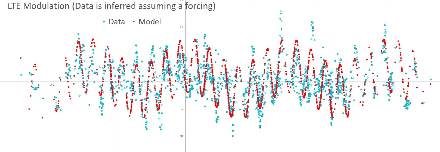
In BLUE again below is a non-linear modulation of the tidal forcing according to the Laplace’s Tidal Equation solution, and trained on an early historical interval. This is something that a neural network should be able to do, as it excels at fitting to non-linear mappings that have a simple (i.e. low complexity) encoding — in this case it may be able to construct a Taylor series expansion of a sinusoidal modulating function.

The neural network’s ability to accurately represent a behavior is explained as a simplicity bias — a confounding aspect of machine learning tools such as ChatGPT and neural networks. The YouTube video below explains the counter-intuitive notion of how a NN with a deep set of possibilities tends to find the simplest solution and doing this without over-fitting the final mapping.

So that deep neural networks are claimed to have a built-in Occam’s Razor propensity, finding the most parsimonious input-output mappings when applied to training data. This is spot on with what I am doing with the LTE mapping, but bypassing the NN with a nonlinear sinusoidal modulation optimally fit on training data by a random search function.

I am tempted to try a NN on the ENSO training set as an experiment and see what it finds.


April 2, 2023

“I am tempted to try a NN on the ENSO training set as an experiment and see what it finds.”

Gerstner waves

An exact solution for equatorially trapped waves
Adrian Constantin, JOURNAL OF GEOPHYSICAL RESEARCH, VOL. 117, C05029, doi:10.1029/2012JC007879, 2012

Nonlinear aspects plays a major role in the understanding of fluid flows. The distinctive fact that in nonlinear problems cause and effect are not proportional opens up the possibility that a small variation in an input quantity causes a considerable change in the response of the system. Often this type of complication causes nonlinear problems to elude exact treatment. A good illustration of this feature is the fact that there is only one known explicit exact solution of the (nonlinear) governing equations for periodic two-dimensional traveling gravity water waves. This solution was first found in a homogeneous fluid by Gerstner

These are trochoidal waves

Even within the context of gravity waves explored in the references mentioned above, a vertical wall is not allowable. This drawback is of special relevance in a geophysical context since [cf. Fedorov and Brown, 2009] the Equator works like a natural boundary and equatorially trapped waves, eastward propagating and symmetric about the Equator, are known to exist. By the 1980s, the scientific community came to realize that these waves are one of the key factors in explaining the El Niño phenomenon (see also the discussion in Cushman-Roisin and Beckers [2011]).

modulo-2π and Berry phase

Cross-Validation of ENSO

Experimenting with linking to slide presentations instead of a trad blog post. The PDF linked below is an eye-opener as the NINO34 fit is the most parsimonious ever, at the expense of a higher LTE modulation (explained here). The cross-validation involves far fewer tidal factors than dealt with earlier, the two factors used (Mf and Mm tidal factors) rivaling the one factor used in QBO (described here).

Continue reading

Information Theory in Earth Science: Been there, done that

Following up from this post, there is a recent sequence of articles in an AGU journal on Water Resources Research under the heading: “Debates: Does Information Theory Provide a New Paradigm for Earth Science?”

By anticipating all these ideas, you can find plenty of examples and derivations (with many centered on the ideas of Maximum Entropy) in our book Mathematical Geoenergy.

Here is an excerpt from the “Emerging concepts” entry, which indirectly addresses negative entropy:

“While dynamical system theories have a long history in mathematics and physics and diverse applications to the hydrological sciences (e.g., Sangoyomi et al., 1996; Sivakumar, 2000; Rodriguez-Iturbe et al., 1989, 1991), their treatment of information has remained probabilistic akin to what is done in classical thermodynamics and statistics. In fact, the dynamical system theories treated entropy production as exponential uncertainty growth associated with stochastic perturbation of a deterministic system along unstable directions (where neighboring states grow exponentially apart), a notion linked to deterministic chaos. Therefore, while the kinematic geometry of a system was deemed deterministic, entropy (and information) remained inherently probabilistic. This led to the misconception that entropy could only exist in stochastically perturbed systems but not in deterministic systems without such perturbations, thereby violating the physical thermodynamic fact that entropy is being produced in nature irrespective of how we model it.

In that sense, classical dynamical system theories and their treatments of entropy and information were essentially the same as those in classical statistical mechanics. Therefore, the vast literature on dynamical systems, including applications to the Earth sciences, was never able to address information in ways going beyond the classical probabilistic paradigm.”

That is, there are likely many earth system behaviors that are highly ordered, but the complexity and non-linearity of their mechanisms makes them appear stochastic or chaotic (high positive entropy) yet the reality is that they are just a complicated deterministic model (negative entropy). We just aren’t looking hard enough to discover the underlying patterns on most of this stuff.

An excerpt from the Occam’s Razor entry, lifts from my cite of Gell-Mann

“Science and data compression have the same objective: discovery of patterns in (observed) data, in order to describe them in a compact form. In the case of science, we call this process of compression “explaining observed data.” The proposed or resulting compact form is often referred to as “hypothesis,” “theory,” or “law,” which can then be used to predict new observations. There is a strong parallel between the scientific method and the theory behind data compression. The field of algorithmic information theory (AIT) defines the complexity of data as its information content. This is formalized as the size (file length in bits) of its minimal description in the form of the shortest computer program that can produce the data. Although complexity can have many different meanings in different contexts (Gell-Mann, 1995), the AIT definition is particularly useful for quantifying parsimony of models and its role in science. “

Parsimony of models is a measure of negative entropy

Inverting non-autonomous functions

This is an algorithm based on minimum entropy (i.e. negative entropy) considerations which is essentially an offshoot of this paper Entropic Complexity Measured in Context Switching.

The objective is to apply negative entropy to find an optimal solution to a deterministically ordered pattern. To start, let us contrast the behavior of autonomous vs non-autonomous differential equations. One way to think about the distinction is that the transfer function for non-autonomous only depends on the presenting input. Thus, it acts like an op-amp with infinite bandwidth. Or below saturation it gives perfectly linear amplification, so that as shown on the graph to the right, the x-axis input produces an amplified y-axis output as long as the input is within reasonable limits.

Continue reading

Nonlinear Generation of Power Spectrum : ENSO

Something I learned early on in my research career is that complicated frequency spectra can be generated from simple repeating structures. Consider the spatial frequency spectra produced as a diffraction pattern produced from a crystal lattice. Below is a reflected electron diffraction pattern of a reconstructed hexagonally reconstructed surface of a silicon (Si) single crystal with a lead (Pb) adlayer ( (a) and (b) are different alignments of the beam direction with respect to the lattice). Suffice to say, there is enough information in the patterns to be able to reverse engineer the structure of the surface as (c).

from link

Now consider the ENSO pattern. At first glance, neither the time-series signal nor the Fourier series power spectra appear to be produced by anything periodically regular. Even so, let’s assume that the underlying pattern is tidally regular, being comprised of the expected fortnightly 13.66 day tropical/synodic cycle and the monthly 27.55 day anomalistic cycle synchronized by an annual impulse. Then the forcing power spectrum of f(t) looks like the RED trace on the left-side of the figure below, F(ω). Clearly that is not enough of a frequency spectra (a few delta spikes) necessary to make up the empirically calculated Fourier series for the ENSO data comprising ~40 intricately placed peaks between 0 and 1 cycles/year in BLUE.

click to expand

Yet, if we modulate that with an Laplace’s Tidal Equation solution functional g(f(t)) that has a G(ω) as in the yellow inset above — a cyclic modulation of amplitudes where g(x) is described by two distinct sine-waves — then the complete ENSO spectra is fleshed out in BLACK in the figure above. The effective g(x) is shown in the figure below, where a slower modulation is superimposed over a faster modulation.

So essentially what this is suggesting is that a few tidal factors modulated by two sinusoids produces enough spectral detail to easily account for the ~40 peaks in the ENSO power spectra. It can do this because a modulating sinusoid is an efficient harmonics and cross-harmonics generator, as the Taylor’s series of a sinusoid contains an effectively infinite number of power terms.

To see this process in action, consider the following three figures, which features a slider that allows one to get an intuitive feel for how the LTE modulation adds richness via harmonics in the power spectra.

  1. Start with a mild LTE modulation and start to increase it as in the figure below. A few harmonics begin to emerge as satellites surrounding the forcing harmonics in RED.
drag slider right for less modulation and to the left for more modulation

2. Next, increase the LTE modulation so that it models the slower sinusoid — more harmonics emerge

3. Then add the faster sinusoid, to fully populate the empirically observed ENSO spectral peaks (and matching the time series).

It appears as if by magic, but this is the power of non-linear harmonic generation. Note that the peak labeled AB amongst others is derived from the original A and B as complicated satellite-cross terms, which can be accounted for by expanding all of the terms in the Taylor’s series of the sinusoids. This can be done with some difficulty, or left as is when doing the fit via solver software.

To complete the circle, it’s likely that being exposed to mind-blowing Fourier series early on makes Fourier analysis of climate data less intimidating, as one can apply all the tricks-of-the-trade, which, alas, are considered routine in other disciplines.


Individual charts

https://imagizer.imageshack.com/img922/7013/VRro0m.png
https://imagizer.imageshack.com/img924/5325/F6Fn4d.png
https://imagizer.imageshack.com/img923/5339/8ErZMz.png
https://imagizer.imageshack.com/img924/4276/wDNlH0.png
https://imagizer.imageshack.com/img924/8150/bXjihg.png
https://imagizer.imageshack.com/img924/6739/C0aNey.png 


The Search for Order

Chap 10 Mathematical Geoenergy

For the LTE formulation along the equator, the analytical solution reduces to g(f(t)), where g(x) is a periodic function. Without knowing what g(x) is, we can use the frequency-domain entropy or spectral entropy of the Fourier series mapping an estimated x=f(t) forcing amplitude to a measured climate index time series such as ENSO. The frequency-domain entropy is the sum or integral of this mapping of x to g(x) in reciprocal space applying the Shannon entropy –I(f).ln(I(f)) normalized over the I(f) frequency range, which is the power spectral (frequency) density of the mapping from the modeled forcing to the time-series waveform sample.

This measures the entropy or degree of disorder of the mapping. So to maximize the degree of order, we minimize this entropy value.

This calculated entropy is a single scalar metric that eliminates the need for evaluating various cyclic g(x) patterns to achieve the best fit. Instead, what it does is point to a highly-ordered spectrum (top panel in the above figure), of which the delta spikes can then be reverse engineered to deduce the primary frequency components arising from the the LTE modulation factor g(x).

The approach works particularly well once the spectral spikes begin to emerge from the background. In terms of a physical picture, what is actually emerging are the principle standing wave solutions for particular wavenumbers. One can see this in the LTE modulation spectrum below where there is a spike at a wavenumber at 1.5 and one at around 10 in panel A (isolating the sin spectrum and cosine spectrum separately instead of the quadrature of the two giving the spectral intensity). This is then reverse engineered as a fit to the actual LTE modulation g(x) in panel B. Panel D is the tidal forcing x=f(t) that minimized the Shannon entropy, thus creating the final fit g(f(t)) in panel C when the LTE modulation is applied to the forcing.

The approach does work, which is quite a boon to the efficiency of iterative fitting towards a solution, reducing the number of DOF involved in the calculation. Prior to this, a guess for the LTE modulation was required and the iterative fit would need to evolve towards the optimal modulation periods. In other words, either approach works, but the entropy approach may provide a quicker and more efficient path to discovering the underlying standing-wave order.

I will eventually add this to the LTE fitting software distro available on GitHub. This may also be applicable to other measures of entropy such as Tallis, Renyi, multi-scale, and perhaps Bispectral entropy, and will add those to the conventional Shannon entropy measure as needed.

Complexity vs Simplicity in Geophysics

In our book Mathematical GeoEnergy, several geophysical processes are modeled — from conventional tides to ENSO. Each model fits the data applying a concise physics-derived algorithm — the key being the algorithm’s conciseness but not necessarily subjective intuitiveness.

I’ve followed Gell-Mann’s work on complexity over the years and so will try applying his qualitative effective complexity approach to characterize the simplicity of the geophysics models described in the book and on this blog.

from Deacon_Information_Complexity_Depth.pdf

Here’s a breakdown from least complex to most complex

Continue reading

Asymptotic QBO Period

The modeled QBO cycle is directly related to the nodal (draconian) lunar cycle physically aliased against the annual cycle.  The empirical cycle period is best estimated by tracking the peak acceleration of the QBO velocity time-series, as this acceleration (1st derivative of the velocity) shows a sharp peak. This value should asymptotically approach a 2.368 year period over the long term.  Since the recent data from the main QBO repository provides an additional acceleration peak from the past month, now is as good a time as any to analyze the cumulative data.


The new data-point provides a longer period which compensated for some recent shorter periods, such that the cumulative mean lies right on the asymptotic line. The jitter observed is explainable in terms of the model, as acceleration peaks are more prone to align close to an annual impulse. But the accumulated mean period is still aligned to the draconic aliasing with this annual impulse. As more data points come in over the coming decades, the mean should vary less and less from the asymptotic value.

The fit to QBO using all the data save for the last available data point is shown below.  Extrapolating beyond the green arrow, we should see an uptick according to the red waveform.


Adding the recent data-point and the blue waveform does follow the model.


There was a flurry of recent discussion on the QBO anomaly of 2016 (shown as a split peak above), which implied that perhaps the QBO would be permanently disrupted from it’s long-standing pattern. Instead, it may be a more plausible explanation that the QBO pattern was not simply wandering from it’s assumed perfectly cyclic path but instead is following a predictable but jittery track that is a combination of the (physically-aliased) annual impulse-synchronized Draconic cycle together with a sensitivity to variations in the draconic cycle itself. The latter calibration is shown below, based on NASA ephermeris.


This is the QBO spectral decomposition, showing signal strength centered on the fundamental aliased Draconic value, both for the data and the set by the model.


The main scientist, Prof. Richard Lindzen, behind the consensus QBO model has been recently introduced here as being “considered the most distinguished living climate scientist on the planet”.  In his presentation criticizing AGW science [1], Lindzen claimed that the climate oscillates due to a steady uniform force, much like a violin oscillates when the steady force of a bow is drawn across its strings.  An analogy perhaps better suited to reality is that the violin is being played like a drum. Resonance is more of a decoration to the beat itself.
Keith 🌛 ?

[1] Professor Richard Lindzen slammed conventional global warming thinking warming as ‘nonsense’ in a lecture for the Global Warming Policy Foundation on Monday. ‘An implausible conjecture backed by false evidence and repeated incessantly … is used to promote the overturn of industrial civilization,’ he said in London. — GWPF