The challenge of validating the models of climate oscillations such as ENSO and QBO, rests primarily in our inability to perform controlled experiments. Because of this shortcoming, we can either do (1) predictions of future behavior and validate via the wait-and-see process, or (2) creatively apply techniques such as cross-validation on currently available data. The first is a non-starter because it’s obviously pointless to wait decades for validation results to confirm a model, when it’s entirely possible to do something today via the second approach.

There are a variety of ways to perform model cross-validation on measured data.

In its original and conventional formulation, cross-validation works by checking one interval of time-series against another, typically by training on one interval and then validating on an orthogonal interval.

Another way to cross-validate is to compare two sets of time-series data collected on behaviors that are potentially related. For example, in the case of ocean tidal data that can be collected and compared across spatially separated geographic regions, the sea-level-height (SLH) time-series data will not necessarily be correlated, but the underlying lunar and solar forcing factors will be closely aligned give or take a phase factor. This is intuitively understandable since the two locations share a common-mode signal forcing due to the gravitational pull of the moon and sun, with the differences in response due to the geographic location and local spatial topology and boundary conditions. For tides, this is a consensus understanding and tidal prediction algorithms have stood the test of time.

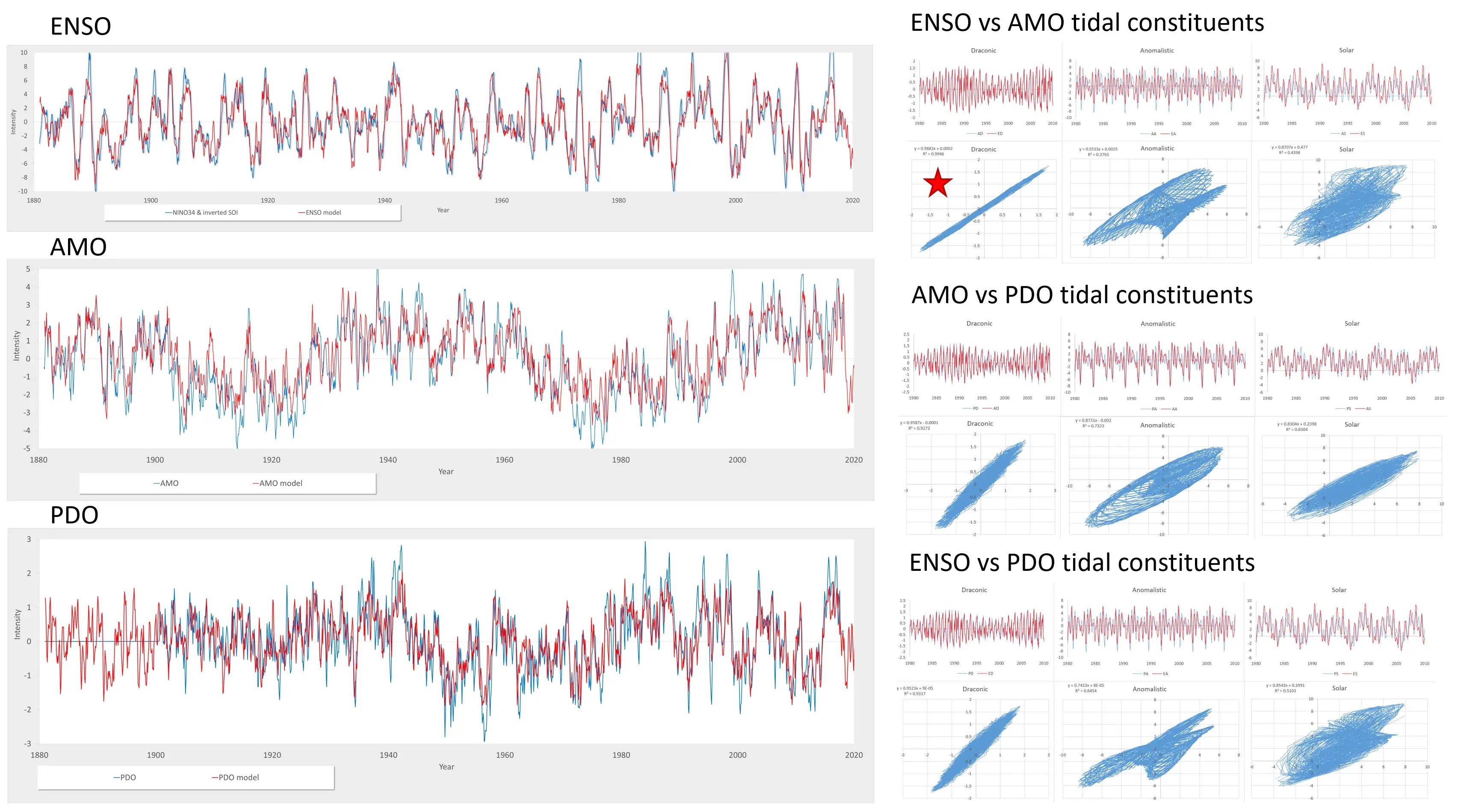
In the previous post, cross-validation on distinct data sets was evaluated assuming common-mode lunisolar forcing. One cross-validation was done between the ENSO time-series and the AMO time-series. Another cross-validation was performed for ENSO against PDO. The underlying common-mode lunisolar forcings were highly correlated as shown in the featured figure.  The LTE spatial wave-number weightings were the primary discriminator for the model fit. This model is described in detail in the book Mathematical GeoEnergy to be published at the end of the year by Wiley.

Another common-mode cross-validation possible is between ENSO and QBO, but in this case it is primarily in the Draconic nodal lunar factor — the cyclic forcing that appears to govern the regular oscillations of QBO.  Below is the Draconic constituent comparison for QBO and the ENSO.

The QBO and ENSO models only show a common-mode correlated response with respect to the Draconic forcing. The Draconic forcing drives the quasi-periodicity of the QBO cycles, as can be seen in the lower right panel, with a small training window.

This cross-correlation technique can be extended to what appears to be an extremely erratic measure, the North Atlantic Oscillation (NAO).

NAO from NOAA https://www.ncdc.noaa.gov/teleconnections/nao/

Like the SOI measure for ENSO, the NAO is originally derived from a pressure dipole measured at two separate locations — but in this case north of the equator.  From the high-frequency of the oscillations, a good assumption is that the spatial wavenumber factors are much higher than is required to fit ENSO. And that was the case as evidenced by the figure below.

ENSO vs NAO cross-validation

Both SOI and NAO are noisy time-series with the NAO appearing very noisy, yet the lunisolar constituent forcings are highly synchronized as shown by correlations in the lower pane. In particular, summing the Anomalistic and Solar constituent factors together improves the correlation markedly, which is because each of those has influence on the other via the lunar-solar mutual gravitational attraction. The iterative fitting process adjusts each of the factors independently, yet the net result compensates the counteracting amplitudes so the net common-mode factor is essentially the same for ENSO and NAO (see lower-right correlation labelled Anomalistic+Solar).

Since the NAO has high-frequency components, we can also perform a conventional cross-validation across orthogonal intervals. The validation interval below is for the years between 1960 and 1990, and even though the training intervals were aggressively over-fit, the correlation between the model and data is still visible in those 30 years.

NAO model fit with validation spanning 1960 to 1990

Over the course of time spent modeling ENSO, the effort that went into fitting to NAO was a fraction of the original time. This is largely due to the fact that the temporal lunisolar forcing only needed to be tweaked to match other climate indices, and the iteration over the topological spatial factors quickly converges.

Many more cross-validation techniques are available for NAO, since there are different flavors of NAO indices available corresponding to different Atlantic locations, and spanning back to the 1800’s.