In Chapter 11 of the book Mathematical GeoEnergy, we model the QBO of equatorial stratospheric winds, but only touch on the related cycle at even higher altitudes, the semi-annual oscillation (SAO). The figure at the top of a recent post geometrically explains the difference between SAO and QBO — the basic idea is that the SAO follows the solar tide and not the lunar tide because of a lower atmospheric density at higher altitudes. Thus, the heat-based solar tide overrides the gravitational lunar+solar tide and the resulting oscillation is primarily a harmonic of the annual cycle.

As can be seen in Fig 1, the semi-annual forcing is by far the strongest and sharpest tidal factor. The symmetry is such that the wind is positive (eastward) whenever the sun is at an equinox nodal crossing and negative (westward) whenever the sun is at a solstice extreme. There is a slight tendency for stronger westward excursions during the southern hemisphere summer.

This solar/tidal generation is the most plausible and parsimonious explanation of the driving force for the SAO, as the alternate explanation of the upper atmosphere creating a resonant frequency of exactly 1/2 year would be preposterously coincidental if true. This also creates a seamless explanation for the source of the lower-altitude QBO, as the synchronized lunar + solar nodal crossings generates the exact required period of 28 months.

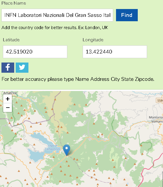
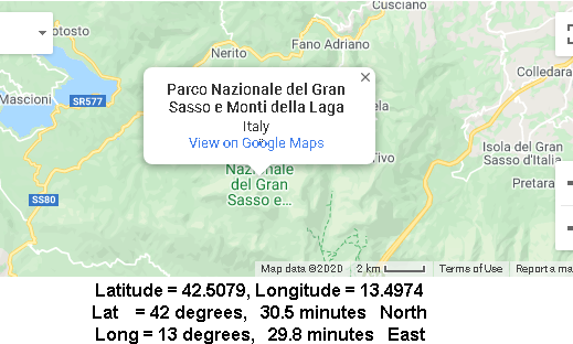
It’s somewhat odd that others have not made the obvious connection of QBO and SAO to the tidal cycles, but even odder is the recent assertion that annual spiky disturbances of the 1 hPa data at northern latitudes (in this case near Sasso in Italy) are caused by invisible dark forces originating from a galactic flux (or something like that) [1].

The authors provide their own geographical explanation as due to a gravitational lensing of cosmic flux, with the disturbances occurring at a specific earth longitudinal alignment and other planets playing a role in the rapid fluctuations within the cone. See the blue horizontal line in the figure below which maps to an average temperature anomaly over a full orbit (one year).

In the Zioutas et al model, if the gravitational focusing occurs at a certain longitude of the earth’s orbit around the sun, then inside the cone the disturbance is sharp as the lens focuses, but outside of this cone of focus, normal seasonal temperature cycles occur.

This annual disturbance at ~1 hPa (about 48 km in altitude) has been observed by others [2]. In the article, von Savigny et al make the remark that these winter disturbances are “mainly due to the action of planetary waves”. Their data originated from near the Eifel mountain region in Germany, and so closely resembles that of Fig 2 in Italy.

To better understand this annual disturbance feature, I downloaded 1 hPa ERA5 reanalysis data from a location close to Sasso, Italy, and used the GEM model fitting algorithm on an average annualized version to match the analysis of Zioutas et al.

Before ascribing this to a cosmic origin, perhaps a more basic question to ask is: What happens if in fact the rapid fluctuations in the annual signal at high-altitudes is simply due to wave breaking?

Fig 5 below shows what happens with strong wave-breaking via a cold impulse and LTE Mach-Zehnder-like modulation occurring near the start of northern latitudes winter.

On the right above is what it would look like without the wave-breaking modulation. The basic ideas that that without wave-breaking, the cooling impulses in December would not break up into multiple high-K waves.

As a simplified model view, consider the modulation shown in the figure to the right. The red profile is an asymmetric seasonal impulse corresponding to a pair of nodal crossings, with one impulse stronger than the other. As the LTE modulation is applied, the resulting blue profile shows a stronger fluctuating disturbance at greater amplitudes.

Another model fit is shown below exclusively using GEM, which takes the annually averaged profile and concatenates them into a time-series to match Fig 4. Because of the properties of LTE modulation, only harmonics of the annual cycle are retained in the training, so that the fine details shown in the fitted model are likely high-K standing wave modes corresponding to the seasonal gravity wave forcing. Relatively few degrees of freedom (DOF) are involved in this model, yet the richness and detail in the data is easily duplicated.

The other possibility is that these disturbances are modulated by lunar tidal cycles as during the observation of SSW events. That this doesn’t appear to be modulated evenly over the entire year is why I find this possibility less plausible than the amplitude-dependent LTE modulation. But either is likely more far more plausible than an invisible space force.

In summary, the SAO at the equator is essentially a balanced sum of the annualized cycles that appear north and south of the equator, creating the semi-annual pattern as the nodal orbit crosses the equator.

At correspondingly lower altitudes, the lunar tides take hold. The figure below is data from a recent paper [3] titled “On the forcings of the unusual Quasi-Biennial Oscillation structure in February 2016“, which like the SAO, may not be as unusual as claimed.

Stay tuned and keep aware, as there’s lots of misleading research being published by AGW skeptics claiming that they understand climate indices.

References

1. Zioutas, K. et al. Stratospheric temperature anomalies as imprints from the dark Universe. Physics of the Dark Universe 28, 100497 (2020).
2. von Savigny, C., Peters, D. H. W. & Entzian, G. Solar 27-day signatures in standard phase height measurements above central Europe. Atmospheric Chemistry and Physics19, 2079–2093 (2019).
3. Li, H., Pilch Kedzierski, R. & Matthes, K. On the forcings of the unusual Quasi-Biennial Oscillation structure in February 2016. Atmospheric Chemistry and Physics 20, 6541–6561 (2020).