Sorry to have to point this out, but it’s not my fault that geophysicists and climatologists can’t perform controlled experiments to test out various hypotheses. It’s not their fault either. It’s all nature’s decision to make gravitational forces so weak and planetary objects so massive to prevent anyone from scaling the effect to laboratory size to enable a carefully controlled experiment. One can always create roughly-equivalent emulations, such as a magnetic field experiment (described in the previous blog post) and validate a hypothesized behavior as a controlled lab experiment. Yet, I suspect that this would not get sufficient buy-in, as it’s not considered the actual real thing.
And that’s the dilemma. By the same token that analog emulators will not be trusted by geophysicists and climatologists, so too scientists from other disciplines will remain skeptical of untestable claims made by earth scientists. If nothing definitive comes out of a thought experiment that can’t be reproduced by others in a lab, they remain suspicious, as per their education and training.
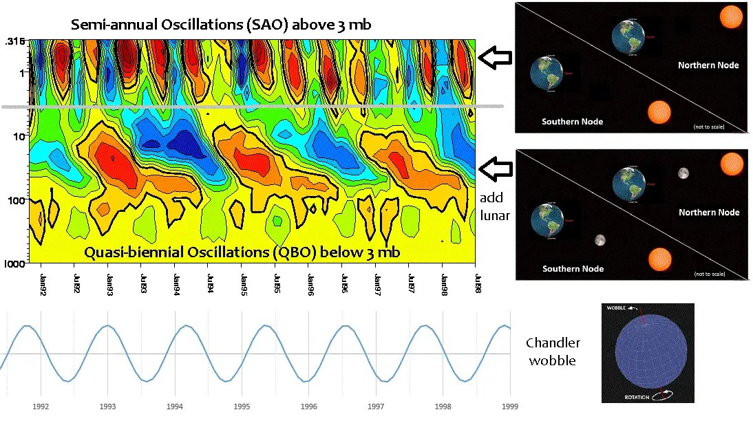
It should therefore work both ways. As featured in the previous blog post, the model of the Chandler wobble forced by lunar torque needs to be treated fairly — either clearly debunked or considered as an alternative to the hazy consensus. ChatGPT remains open about the model, not the least bit swayed by colleagues or tribal bias. As the value of the Chandler wobble predicted by the lunar nodal model (432.7 days) is so close to the cited value of 433 days, as a bottom-line it should be difficult to ignore.

There are other indicators in the observational data to further substantiate this, see Chandler Wobble Forcing. It also makes sense in the context of the annual wobble.
As it stands, the lack of an experiment means a more equal footing for the alternatives, as they are all under equal amounts of suspicion.
Same goes for QBO. No controlled experiment is possible to test out the consensus QBO models, despite the fact that the Plumb and McEwan experiment is claimed to do just that. Sorry, but that experiment is not even close to the topology of a rotating sphere with a radial gravitational force operating on a gas. It also never predicted the QBO period. In contrast, the value of the QBO predicted by the lunar nodal model (28.4 months) is also too close to the cited value of 28 to 29 months to ignore. This also makes sense in the context of the semi-annual oscillation (SAO) located above the QBO .

Both the Chandler wobble and the QBO have the symmetry of a global wavenumber=0 phenomena so therefore only nodal cycles allowed — both for lunar and solar.
Next to ENSO. As with LOD modeling, this is not wavenumber=0 symmetry, as it must correspond to the longitude of a specific region. No controlled experiment is possible to test out the currently accepted models, premised as being triggered by wind shifts (an iffy cause vs. effect in any case). The mean value of the ENSO predicted by the tidal LOD-caibrated model (3.80 years modulated by 18.6 years) is too close to the cited value of 3.8 years with ~200 years of paleo and direct measurement to ignore.

doi:10.1007/978-1-4020-4411-3_172
In BLUE below is the LOD-calibrated tidal forcing, with linear amplification

In BLUE again below is a non-linear modulation of the tidal forcing according to the Laplace’s Tidal Equation solution, and trained on an early historical interval. This is something that a neural network should be able to do, as it excels at fitting to non-linear mappings that have a simple (i.e. low complexity) encoding — in this case it may be able to construct a Taylor series expansion of a sinusoidal modulating function.

The neural network’s ability to accurately represent a behavior is explained as a simplicity bias — a confounding aspect of machine learning tools such as ChatGPT and neural networks. The YouTube video below explains the counter-intuitive notion of how a NN with a deep set of possibilities tends to find the simplest solution and doing this without over-fitting the final mapping.
So that deep neural networks are claimed to have a built-in Occam’s Razor propensity, finding the most parsimonious input-output mappings when applied to training data. This is spot on with what I am doing with the LTE mapping, but bypassing the NN with a nonlinear sinusoidal modulation optimally fit on training data by a random search function.
I am tempted to try a NN on the ENSO training set as an experiment and see what it finds.
April 2, 2023
“I am tempted to try a NN on the ENSO training set as an experiment and see what it finds.”