The harmonics generator of the ocean

The research category is topological considerations of Laplace’s Tidal Equations (LTE = a shallow-water simplification of Navier-Stokes) applied to the equatorial thermocline — the following citations provides an evolutionary understanding that I have developed via presentations and publications over the last 6 years (working backwards)

“Nonlinear long-period tidal forcing with application to ENSO, QBO, and Chandler wobble”, EGU General Assembly Conference Abstracts, 2021, EGU21-10515
ui.adsabs.harvard.edu/abs/2021EGUGA..2310515P/abstract

“Nonlinear Differential Equations with External Forcing”, ICLR 2020 Workshop DeepDiffEq 
https://openreview.net/forum?id=XqOseg0L9Q

“Mathematical Geoenergy: Discovery, Depletion, and Renewal”, John Wiley & Sons, 2019, chapter 12: “Wave Energy” 
https://agupubs.onlinelibrary.wiley.com/doi/10.1002/9781119434351.ch12

“Ephemeris calibration of Laplace’s tidal equation model for ENSO”, AGU Fall Meeting 2018, 
https://www.essoar.org/doi/abs/10.1002/essoar.10500568.1

“Biennial-Aligned Lunisolar-Forcing of ENSO: Implications for Simplified Climate Models”,
AGU Fall Meeting 2017, https://www.essoar.org/doi/abs/10.1002/essoar.b1c62a3df907a1fa.b18572c23dc245c9.1

“Analytical Formulation of Equatorial Standing Wave Phenomena: Application to QBO and ENSO”, AGU Fall Meeting Abstracts 2016, OS11B-04, 
ui.adsabs.harvard.edu/abs/2016AGUFMOS11B..04P/abstract

Given that I have worked on this topic persistently over this span of time, I have gained considerable insight into how straightforward it has become to generate relatively decent fits to climate dipoles such as ENSO. Paradoxically, this is both good and bad. It’s good because the model’s recipe is algorithmically simply described in terms of plausibility and parsimony. That’s largely because it’s a straightforward non-linear extension of a conventional tidal analysis model. However that non-linearity opens up the possibility for many similar model fits that are equally good, yet difficult to discriminate between. So it’s bad in the sense that I can come to an impasse in selecting the “best” model.

This is oversimplifying a bit but the framing issue is if you knew the answer was 72, but have a hard time determining whether the question being posed was one of 2×36, 3×24, 4×18, 6×12, 8×9, 9×8, 12×6, 18×4, 24×3, or 36×2. Each gives the right answer, but potentially not the right mechanism. This is a fundamental problem with non-linear analysis.

A conventional tidal analysis by itself is just a few fundamental tidal factors (exactly 4) but made devastatingly accurate by the introduction of 2nd-order harmonics and cross-harmonics. All these harmonics are generated by non-linear effects but the frequency spectrum is so clean and distinct for a sea-level-height (SLH) time-series that the equivalent solution to k × F = 72 is essentially a scaling identification problem where the k is the scale factor for the corresponding cyclic tidal factors F.

Yet, by applying the non-linear LTE solution to the problem of modeling ENSO, we quickly discover that the algorithm is a wickedly effective harmonics and cross-harmonics generator. Any number of combinations of harmonics can develop an adequate fit depending on the variable LTE modulation applied. So it could be a small LTE modulation mixed with a wide assortment of tidal factors (the 2×36 case) or it could be a large LTE modulation mixed with a minimum of tidal factors (the 18×4 case). Or it could be something in between (e.g. the 8×9 case). This is all a result of the sine-of-a-sine non-linearity of the LTE formulation, related to the Mach-Zehnder modulation used in optical cryptography applications. The latter bit is the hint that things may not be unambiguously decoded given the fact that M-Z has been discovered to be nature’s own built-in encryption device.

However, there remains lots of light at the end of this tunnel, as I have also discovered that the tidal factor spread is likely largely governed by a single lunar tidal constituent, the 27.55 day anomalistic Mm cycle interfering with an annual impulse. That’s essentially 2 of the 4 tidal factors, with the other 2 lunar factors providing a 2nd-order correction. For the longest time I had been focused on the 13.66 day tropical Mf cycle as that also lead to a decent fit over the years, specifically since the first beat harmonic of the Mf cycle with the annual impulse is 3.8 years while the Mm cycle is 3.9 years. These two terms are close enough that they only go out-of-phase after ~130 years, which is the extent of the ENSO time-series. Only when you try to simplify a model fit by iterating over the space of factor combinations will you discover the difference between 3.8 and 3.9.

In terms of geophysics, the Mf factor is a tractional tidal forcing operating parallel to the ocean’s surface influenced by the moon’s latitudinal declination, while the Mm factor is a largely perpendicular gravitational forcing influenced by the perigean cycle of the Moon-to-Earth distance. The latter may be the “right mechanism” as each can give close to the “right answer”.

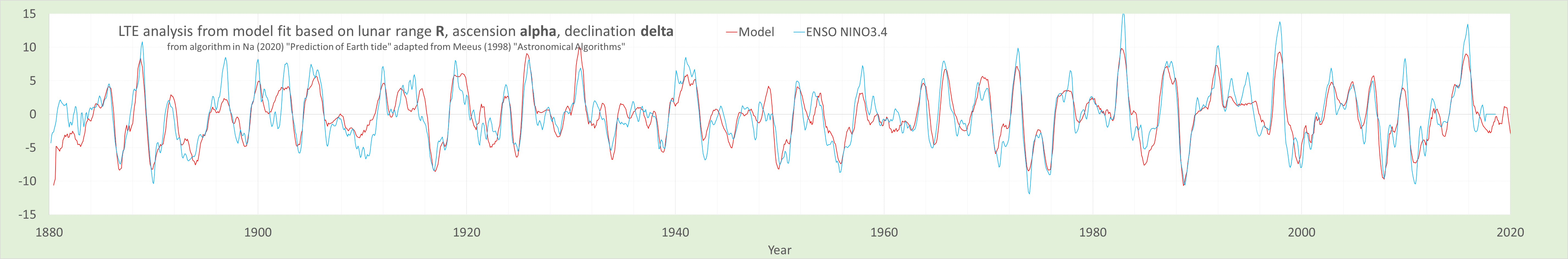
So the gist of the fitting observations is that far fewer harmonic factors are required for a decent Mm-based model than for a Mf-based model. This is slightly at the expense of a stronger LTE modulation, but the parsimony of an Mm-based model can’t be beat, as I will show via the following analysis charts…

This is a good model fit based on a slightly modified Mm-based factorization, with a sample-and-hold placed on a strong annual impulse

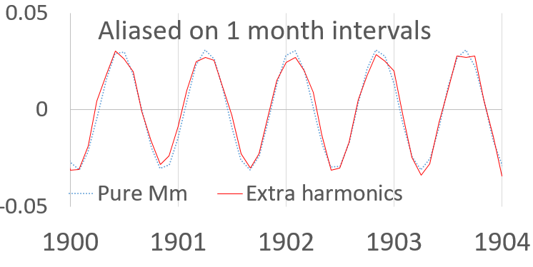
The comparison of the modified Mm tidal factorization to the pure Mm is below (the reason the 27.55 day periodicity doesn’t appear is because of the monthly aliasing used in plotting).

The slight pattern on top of pure signal is due to a 6-year beat of the Mm period with the 27.212 day lunar draconic pattern indicating the time between equatorial nodal crossings of the moon. This is the strongest factor of the ascension cycle described in the solar and lunar ephemeris published recently by Sung-Ho Na. As highlighted above by numbered cycles, ~20 occur in the span of 120 years.

Below, an expanded look showing how slight a correction is applied

The integrated forcing after the annual impulse is shown below. The sample-and-hold integration exaggerates low-frequency differences so the distinction between the pure Mm forcing and Mm+harmonics is more apparent. The 6-year periodicity is obscured by longer term variations.

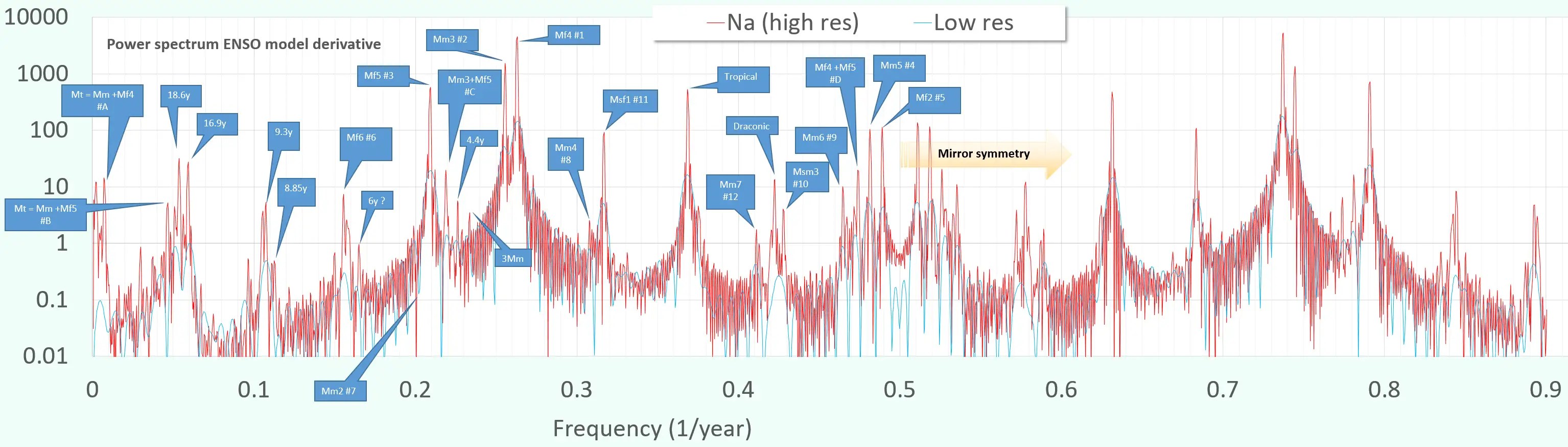
The log-scaled power spectra of the integrated tidal forcing is shown below. Note the overwhelmingly strong peak near the 0.25/year frequency (3.9 year cycle). The rest of the peaks are readily matched to periodicities in the Na ephemerides [1] according to their strength.

The LTE modulation is quite strong for this factorization. As shown below, the forcing levels need to sinusoidally fold several times over to match the observed ENSO behavior. See the recent post Inverting non-autonomous functions for a recipe to aid in iterating for the underlying LTE modulation.

The parsimony of this model can’t be emphasized enough. It’s equivalent to the agreement of a conventional tidal forcing analysis to a SLH time-series in that only a single lunar tidal factor accounts for a majority of the modulation. Only the challenge of finding the correct LTE modulation stands in the way of producing an unambiguously correct model for the underlying ENSO behavioral dynamics.

References

[1] Sung-Ho Na, Chapter 19 – Prediction of Earth tide, Editor(s): Pijush Samui, Barnali Dixon, Dieu Tien Bui, Basics of Computational Geophysics, Elsevier, 2021, Pages 351-372, ISBN 9780128205136,
https://doi.org/10.1016/B978-0-12-820513-6.00022-9. (note: the ephemerides for the Earth-Moon-Sun system matches closely the online NASA JPL ephemerides generator available at https://ssd.jpl.nasa.gov/horizons, but this paper is more useful in that it algorithmically states the contributions of the various tidal factors in the source code supplied. Source code also available at https://github.com/pukpr/GeoEnergyMath/tree/master/src)


Myth: El Nino/La Nina transitions caused by wind

This 2-D heat map, from Jialin Lin’s research group at The Ohio State University, shows the eastward propagation of the ocean subsurface wave leading to switch from La Niña to El Niño.

The above is from an informative OSU press release from last year titled Solving climate’s toughest questions, one challenge at a time. The following quotes are from that page, bold emphasis mine.

Jialin Lin, associate professor of geography, has spent the last two decades tackling those challenges, and in the past two years, he’s had breakthroughs in answering two of forecasting’s most pernicious questions: predicting the shift between El Niño and La Niña and predicting which hurricanes will rapidly intensify.

Now, he’s turning his attention to creating more accurate models predicting global warming and its impacts, leading an international team of 40 climate experts to create a new book identifying the highest-priority research questions for the next 30-50 years.

… still to be published

Lin set out to create a model that could accurately identify ENSO shifts by testing — and subsequently ruling out — all the theories and possibilities earlier researchers had proposed. Then, Lin realized current models only considered surface temperatures, and he decided to dive deeper.

He downloaded 140 years of deep-ocean temperature data, analyzed them and made a breakthrough discovery.

“After 20 years of research, I finally found that the shift was caused by an ocean wave 100 to 200 meters down in the deep ocean,” Lin said, whose research was published in a Nature journal. “The propagation of this wave from the western Pacific to the eastern Pacific generates the switch from La Niña to El Niño.”

The wave repeatedly appeared two years before an El Niño event developed, but Lin went one step further to explain what generated the wave and discovered it was caused by the moon’s tidal gravitational force.

“The tidal force is even easier to predict,” Lin said. “That will widen the possibility for an even longer lead of prediction. Now you can predict not only for two years before, but 10 years before.”

Essentially, the idea is that these subsurface waves can in no way be caused by surface wind as the latter only are observed later (likely as an after-effect of the sub-surface thermocline nearing the surface and thus modifying the atmospheric pressure gradient). This counters the long-standing belief that ENSO transitions occur as a result of prevailing wind shifts.

The other part of the article concerns correlating hurricane intensification is also interesting.

p.s. It’s all tides : Climatic Drivers of Extreme Sea Level Events Along the
Coastline of Western Australia

Information Theory in Earth Science: Been there, done that

Following up from this post, there is a recent sequence of articles in an AGU journal on Water Resources Research under the heading: “Debates: Does Information Theory Provide a New Paradigm for Earth Science?”

By anticipating all these ideas, you can find plenty of examples and derivations (with many centered on the ideas of Maximum Entropy) in our book Mathematical Geoenergy.

Here is an excerpt from the “Emerging concepts” entry, which indirectly addresses negative entropy:

“While dynamical system theories have a long history in mathematics and physics and diverse applications to the hydrological sciences (e.g., Sangoyomi et al., 1996; Sivakumar, 2000; Rodriguez-Iturbe et al., 1989, 1991), their treatment of information has remained probabilistic akin to what is done in classical thermodynamics and statistics. In fact, the dynamical system theories treated entropy production as exponential uncertainty growth associated with stochastic perturbation of a deterministic system along unstable directions (where neighboring states grow exponentially apart), a notion linked to deterministic chaos. Therefore, while the kinematic geometry of a system was deemed deterministic, entropy (and information) remained inherently probabilistic. This led to the misconception that entropy could only exist in stochastically perturbed systems but not in deterministic systems without such perturbations, thereby violating the physical thermodynamic fact that entropy is being produced in nature irrespective of how we model it.

In that sense, classical dynamical system theories and their treatments of entropy and information were essentially the same as those in classical statistical mechanics. Therefore, the vast literature on dynamical systems, including applications to the Earth sciences, was never able to address information in ways going beyond the classical probabilistic paradigm.”

That is, there are likely many earth system behaviors that are highly ordered, but the complexity and non-linearity of their mechanisms makes them appear stochastic or chaotic (high positive entropy) yet the reality is that they are just a complicated deterministic model (negative entropy). We just aren’t looking hard enough to discover the underlying patterns on most of this stuff.

An excerpt from the Occam’s Razor entry, lifts from my cite of Gell-Mann

“Science and data compression have the same objective: discovery of patterns in (observed) data, in order to describe them in a compact form. In the case of science, we call this process of compression “explaining observed data.” The proposed or resulting compact form is often referred to as “hypothesis,” “theory,” or “law,” which can then be used to predict new observations. There is a strong parallel between the scientific method and the theory behind data compression. The field of algorithmic information theory (AIT) defines the complexity of data as its information content. This is formalized as the size (file length in bits) of its minimal description in the form of the shortest computer program that can produce the data. Although complexity can have many different meanings in different contexts (Gell-Mann, 1995), the AIT definition is particularly useful for quantifying parsimony of models and its role in science. “

Parsimony of models is a measure of negative entropy

Odd cycles in Length-of-Day (LOD) variations

Two papers on the analysis of >1 year periods in the LOD time series measured since 1962.

The consistency of interdecadal changes in the Earth’s rotation variations

On the ~ 7 year periodic signal in length of day from a frequency domain stepwise regression method

These cycles may be related to aliased tidal periods with the annual cycle, as in modeling ENSO.


A paper describing new satellite measurements for precision LOD measurements.

BeiDou satellite radiation force models for precise orbit
determination and geodetic applications
” from TechRxiv

Note the detail on the 13.6 day fortnightly tidal period

“Wobbling” Moon trending on Twitter

Twitter trending topic

This NASA press release has received mainstream news attention.

The 18.6 year nodal cycle will generate higher tides that will exaggerate sea-level rise due to climate change.

Yahoo news item:

https://news.yahoo.com/lunar-orbit-apos-wobble-apos-173042717.html

So this is more-or-less a known behavior, but hopefully it raises awareness to the other work relating lunar forcing to ENSO, QBO, and the Chandler wobble.

Cited paper

Thompson, P.R., Widlansky, M.J., Hamlington, B.D. et al. Rapid increases and extreme months in projections of United States high-tide flooding. Nat. Clim. Chang. 11, 584–590 (2021). https://doi.org/10.1038/s41558-021-01077-8

Inverting non-autonomous functions

This is an algorithm based on minimum entropy (i.e. negative entropy) considerations which is essentially an offshoot of this paper Entropic Complexity Measured in Context Switching.

The objective is to apply negative entropy to find an optimal solution to a deterministically ordered pattern. To start, let us contrast the behavior of autonomous vs non-autonomous differential equations. One way to think about the distinction is that the transfer function for non-autonomous only depends on the presenting input. Thus, it acts like an op-amp with infinite bandwidth. Or below saturation it gives perfectly linear amplification, so that as shown on the graph to the right, the x-axis input produces an amplified y-axis output as long as the input is within reasonable limits.

Continue reading

Low #DOF ENSO Model

Given two models of a physical behavior, the “better” model has the highest correlation (or lowest error) to the data and the lowest number of degrees of freedom (#DOF) in terms of tunable parameters. This ratio CC/#DOF of correlation coefficient over DOF is routinely used in automated symbolic regression algorithms and for scoring of online programming contests. A balance between a good error metric and a low complexity score is often referred to as a Pareto frontier.

So for modeling ENSO, the challenge is to fit the quasi-periodic NINO34 time-series with a minimal number of tunable parameters. For a 140 year fitting interval (1880-1920), a naive Fourier series fit could easily take 50-100 sine waves of varying frequencies, amplitudes, and phase to match a low-pass filtered version of the data (any high-frequency components may take many more). However that is horribly complex model and obviously prone to over-fitting. Obviously we need to apply some physics to reduce the #DOF.

Since we know that ENSO is essentially a model of equatorial fluid dynamics in response to a tidal forcing, all that is needed is the gravitational potential along the equator. The paper by Na [1] has software for computing the orbital dynamics of the moon (i.e. lunar ephemerides) and a 1st-order approximation for tidal potential:

The software contains well over 100 sinusoidal terms (each consisting of amplitude, frequency, and phase) to internally model the lunar orbit precisely. Thus, that many DOF are removed, with a corresponding huge reduction in complexity score for any reasonable fit. So instead of a huge set of factors to manipulate (as with many detailed harmonic tidal analyses), what one is given is a range (r = R) and a declination ( ψ=delta) time-series. These are combined in a manner following the figure from Na shown above, essentially adjusting the amplitudes of R and delta while introducing an additional tangential or tractional projection of delta (sin instead of cos). The latter is important as described in NOAA’s tide producing forces page.

Although I roughly calibrated this earlier [2] via NASA’s HORIZONS ephemerides page (input parameters shown on the right), the Na software allows better flexibility in use. The two calculations essentially give identical outputs and independent verification that the numbers are as expected.

As this post is already getting too long, this is the result of doing a Laplace’s Tidal Equation fit (adding a few more DOF), demonstrating that the limited #DOF prevents over-fitting on a short training interval while cross-validating outside of this band.

or this

This low complexity and high accuracy solution would win ANY competition, including the competition for best seasonal prediction with a measly prize of 15,000 Swiss francs [3]. A good ENSO model is worth billions of $$ given the amount it will save in agricultural planning and its potential for mitigation of human suffering in predicting the timing of climate extremes.

REFERENCES

[1] Na, S.-H. Chapter 19 – Prediction of Earth tide. in Basics of Computational Geophysics (eds. Samui, P., Dixon, B. & Tien Bui, D.) 351–372 (Elsevier, 2021). doi:10.1016/B978-0-12-820513-6.00022-9.

[2] Pukite, P.R. et al “Ephemeris calibration of Laplace’s tidal equation model for ENSO” AGU Fall Meeting, 2018. doi:10.1002/essoar.10500568.1

[3] 1 CHF ~ $1 so 15K = chump change.


Added: High resolution power spectra of ENSO forcing
see link

Nonlinear long-period tidal forcing with application to ENSO, QBO, and Chandler wobble

Model fitting process for ENSO

Back to EGU abstract and presentation


Addendum: After this presentation was submitted, a ground-breaking paper by a group at the University of Paris came on-line. Their paper, “On the Shoulders of Laplace” covers much the same ground as the EGU presentation linked above.

Their main thesis is that Pierre-Simon Laplace in 1799 correctly theorized that the wobble in the Earth’s rotation is due to the moon and sun, described in the treatise “Traité de Mécanique Céleste (Treatise of Celestial Mechanics)“.


Excerpts from the paper “On the shoulders of Laplace”

Moreover Lopes et al claim that this celestial gravitational forcing carries over to controlling cyclic climate indices, following Laplace’s mathematical formulation (now known as Laplace’s Tidal Equations) for describing oceanic tides.

Excerpt from the paper “On the shoulders of Laplace”

This view also aligns with the way we model climate indices such as ENSO and QBO via a solution to Laplace’s Tidal Equations, as described in the linked EGU presentation above.