[mathjax]After playing around with the best way to map a model to ENSO, I am coming to the conclusion that the wave equation transformation is a good approach.

Fig. 1: Upper is the wave transformation fit to SOI, lower is the difference error signal, very uniform and flat.
What the transformation amounts to is a plot of the LHS vs the RHS of the SOI differential wave equation, where k(t) (the Mathieu or Hill factor) is estimated corresponding to a characteristic frequency of ~1/(4 years),
$$ SOI”(t)+k(t) SOI(t) = F(t) $$
and where F(t) is the forcing function, comprised of the main suspects of QBO, Chandler wobble, TSI, and the long term tidal beat frequencies.
I added a forcing break at 1980, likely due to TSI, to get the full 1880 to 2013 fit.
The wavelet scalogram agreement is very impressive, indicating that all frequency scales are being accounted for.
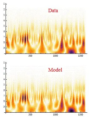
Fig 2: Wavelet scalogram, scale in months since 1880.
This is essentially just a different way of looking at the model described in the ARXIV ENSO sloshing paper. What one can do is extend the forcing and then do an integration of the LHS to project the ENSO waveform into the future.

Pingback: Eureqa! | context/Earth
Pingback: Presentation at AGU 2016 on December 12 | context/Earth
Pingback: Solution to Pulsed Mathieu Equation | context/Earth
Pingback: Canonical Solution of Mathieu Equation for ENSO | context/Earth