[mathjax]An old game show called Name That Tune asked contestants to identify a song by listening to just a few notes.
This post is the QBO equivalent to that. How short an interval can we train on to reproduce the rest of the time series? The answer is not much is required.
Using only three fundamental frequencies on the QBO acceleration: (1) the strong aliased Draconic, (2) an annual signal, and (3) a semi-annual signal, the rest of the data can be fit by using an interval as short as 3 to 4 years. The aliased Draconic signal is 2.36 years with the accompanying harmonics at 0.292, 0.413, 0.703, 1.73, 0.634 that sharpen the peaks on a seasonal basis.
| Aliased Harmonic | Frequency | Period |
| Y/27.212-10 | 3.423 | 0.292 |
| Y/27.212-11 | 2.423 | 0.413 |
| Y/27.212-12 | 1.423 | 0.703 |
| Y/27.212-13 | 0.423 | 2.363 |
| Y/27.212-14 | -0.577 | -1.734 |
| Y/27.212-15 | -1.577 | -0.634 |
| Y/27.212-16 | -2.577 | -0.388 |
Where Y is the year in days. The shorter periods provide the fine structure and help to isolate the tidal frequency as they sharpen and define the acceleration peak amplitude on such a short interval (Figure 1).

Fig. 1: Training from 1978 to 1982 highlighted in yellow
The following training interval runs from 1970 to 1974 (Figure 2). Even though it trains on a different interval, the results on the validation interval looks very similar to the previous result of Figure 1! This indicates that there is an intrinsic stationary behavior common to the two intervals.
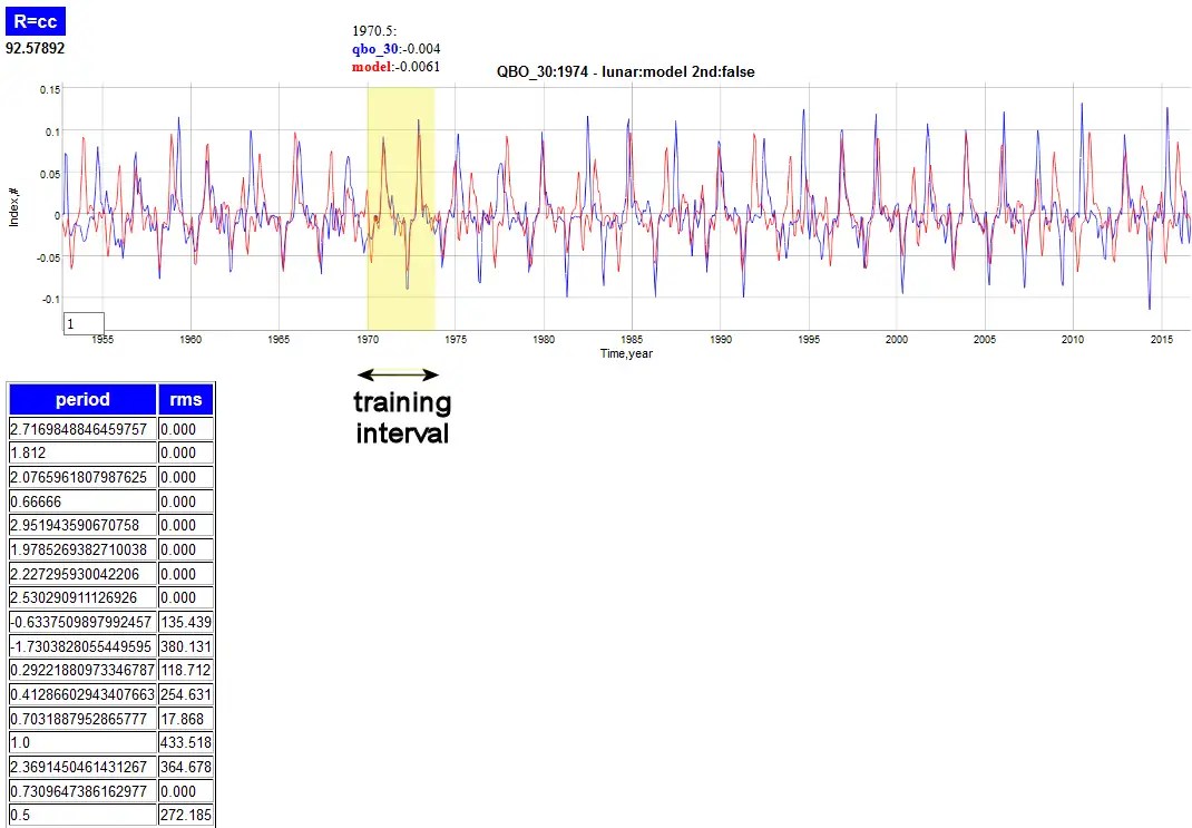
Fig. 2: Training from 1970 to 1974 highlighted in yellow.
If one looks closely, the amount of detail that is replicated in the data by the model is also quite intricate in places. Yet there are intervals that show shifts in the peaks. It’s possible that some of the acceleration peaks are shifted due to transient volcanic effects on the stratosphere. Look at the discrepancy regions in yellow below and we can determine which may be associated with volcanic events.
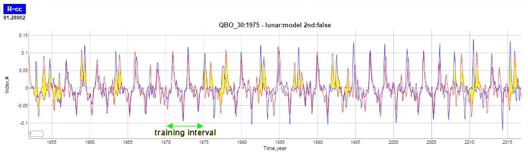
Fig. 3: Discrepancies highlighted in yellow. Are their particular geophysical events associated with these regions?
So far the training intervals happen to be regions that are free of significant volcanic eruptions. The following fit also uses a largely volcano-free training interval from 1996-2006 and one can see the three significant volcanic events of the 20th century ( Agung – 1963, El Chichon – 1982, Pinatubo – 1991) immediately preceded regions that show discrepancy between the model fit and the data (the regions in yellow ♦).

Fig. 4: For a training interval from 1996 to 2006, the yellow-shaded regions indicate potential perturbations caused by volcanic events
In general, any deviations are likely due to whether the seasonal tidal impulse is enough to trigger the QBO reversal during that Draconic lunar cycle or a subsequent one. So it is possible that volcanic particulates released to the stratosphere could impact the temperature of the layer, thus speeding up onset of a warm season, or delaying the transition to a cool season.
Importantly, we did not apply the Tropical and Anomalous lunar cycles to the fit, which could potentially improve the timing. But this would also require a longer training interval to avoid the problems of overfitting. The following is an Excel fit using the Solver plug-in where the Draconic lunar period was allowed to vary. The regions denoted by the blue horizontal bars were used as training intervals. Using the GRG Nonlinear solving method, the best fit for the Draconic period was 27.211 days, which compares favorably to the known value of 27.212 days (Figure 5). The difference of 0.001 day accumulates to less than a day over 50 years.

Fig 5: Excel solver fit of the Draconic period. Lower panel is the difference between model (red) and data (blue). Intervals defined by horizontal bars are the non-volcanic intervals.
Another important point to note if these are indeed volcanic disturbances impacting the transient behavior, is that the QBO regains phase alignment with the lunar tides relatively quickly — as if it had no long-term effect. This is a hallmark of an ergodic process forcibly driven by a guiding temporal boundary condition.
Also worth noting is that such a limited data series would have allowed Richard Lindzen to do this exercise back in the 1960’s and thus potentially project the QBO behavior over the ensuing years. And that also implies he provided poor guidance to our understanding of QBO. Consider how many papers are trying to explain the recent QBO anomaly. The fact that volcanic events, ENSO timing, and AGW could each impact the seasonal impact of the tidal forcing, having a solid foundational model for the stationary behavior is critical.
UPDATE – 10/11/2016
I fed the 1970-1974 and 1996-2006 QBO‘ 30-hPa training intervals into a symbolic regression machine learning tool to see what it would uncover, shown below.
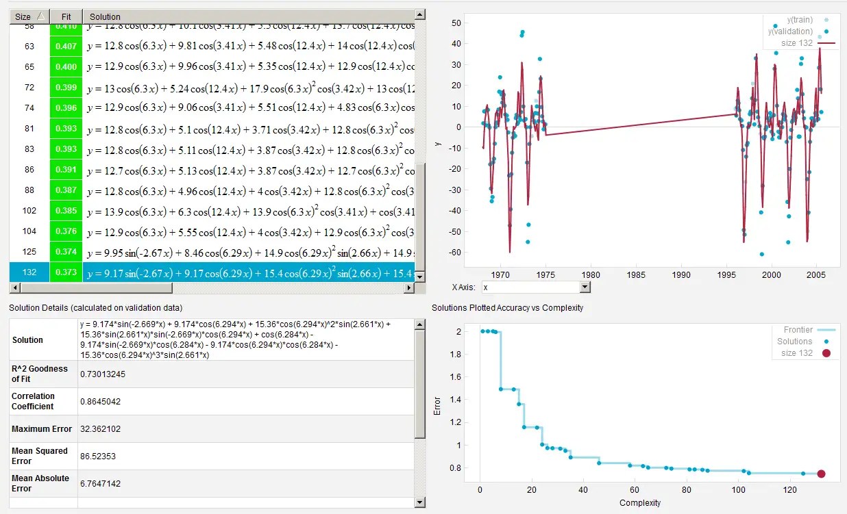
Fig 6 : Machine learning Pareto front. The empty gap between the two data sets is ignored by the algorithm, yet an artifactual straight line connects the two. The highest complexity and smallest error solution was selected.
The solution contains the ~2.66 rad/year fundamental with harmonics that are aliased multiples of $$2pi$$ rad/year spaced from that. In particular, from an expanded view of the solution (by refactoring the $$cos(2pi x)^N$$ terms), the multiples range from $$-6pi$$, $$-4pi$$, $$-2pi$$, $$2pi$$, $$4pi$$, $$6pi$$. There is also a non-aliased harmonic of 2.66, i.e. precisely double that frequency, which is also predicted by the QBO cos(sin(wt)+constant) model. Any asymmetries in positive versus negative excursions will typically reveal that harmonic.

Fig 7 : Focus on machine learning results.
| Aliased Harmonic | Frequency (1/y) |
Period (y) |
| 2.66 + $$6pi$$ | 3.423 | 0.292 |
| 2.66 + $$4pi$$ | 2.423 | 0.413 |
| 2.66 + $$2pi$$ | 1.423 | 0.703 |
| 2.66 = main harmonic | 0.423 | 2.363 |
| 2.66 – $$2pi$$ | -0.577 | -1.734 |
| 2.66 – $$4pi$$ | -1.577 | -0.634 |
| 2.66 – $$6pi$$ | -2.577 | -0.388 |
The important point to note is that the table at the top of this post and the machine learning results are the same! Let that sink in. The top table was filled in based on the physical knowledge of aliasing the 27.212 day Draconic lunar tide against an annual signal would produce those specific harmonics. The bottom table was filled in by a symbolic reasoning engine finding the same terms by exhaustively testing millions of possibilities for the best and most canonical fit — only assuming that y = f(x), a completely arbitrary function. In other words, the machine learning knows nothing about the physics yet finds the same set of terms.
As a second check, the closed form expression produced by the symbolic regression also fits right on top of the model optimized by the Excel solver.
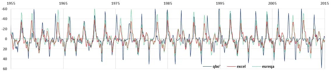
Fig 8 : The model (excel in red) lies on top of the symbolic regression machine learning result (eureqa in green). The blue is the QBO acceleration data.
As far as a finishing touch, it will not be difficult to add an impulse response to this model to fit the volcanic disturbances. This will presumably apply the Sato stratospheric aerosol model to generate the appropriate delta functions.

The specific machine learning app will never generate the same result twice so it is of limited use in terms of scientific reproducibility. Here is another solution with not as good a correlation with the data:
If you want to pay thousands of $ to purchase a license and reproduce the results, knock yourself out.
LikeLike
In this experiment, I let the machine learning run overnight. 1.3 trillion formula evaluations later …
Not that in the following, it picked out a factor 3.632 rads/year which is 365.242/(14 – 3.632 / $$2\pi$$) = 27.2123 days.
That is way too significant given the short span but the Draconic lunar month is 27.2122 days
LikeLike
Have you looked at Isaac Held’s latest blog post? 72. Odd recent evolution of the QBO.
LikeLike
Thanks Kevin,
That explanation for QBO makes my brain hurt. He should be able to demonstrate the behavior mathematically.
LikeLike
It’s not so much his explanation, but the fact the QBO is behaving oddly. Sam Lillo’s MQI Phase Space plots show the anomaly visually:
Is this behavior also different from what your model would predict?
LikeLike
Thanks. I will have to understand what he is plotting before I can deduce what exactly is different.
LikeLike
Pingback: Short Training Intervals for ENSO | context/Earth
Pingback: Presentation at AGU 2016 on December 12 | context/Earth
Pingback: Confirmation Bias | context/Earth