In Chapter 11 and Chapter 12 of the book we characterize deterministic and stochastic variability in waves. While reviewing the presentations at last week’s EGU meeting, one study covered some of the same ground [1] and was worth a more detailed look. The distribution of stratospheric wind wave energy collected by Nastrom [2] (shown below) that we model in Chapter 11 is apparently still not completely understood.

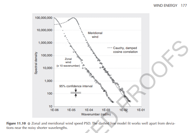
They present it as below, with the caveat that the tailing off at high wavenumber (or shorter wavelength) disperses with a k^-5/3 dependence referred to Kologorov’s 5/3 spectrum and arising due to turbulence, though still controversial as the authors claim in the bullet points.

In our interpretation, the piece-wise power-law roll-off shown above is replaced by a smooth continuum with inflection points determined by the specific shape of the Cauchy density function. The Cauchy characterizes a stochastic distribution of some mix of standing and traveling wavetrains, with a preferred wavenumber defined by the cusp location. This disordered distribution is in contrast to the highly ordered nature of the QBO and of standing waves in a constrained container.

The continuum from deterministic to stochastic is essentially described as:

• Highly ordered deterministic waves, potentially including harmonics (see QBO with characteristic squared off waves)
• A specific amount of disorder applied as a semi-Markov process, maintaining harmonics
• Dispersion applied to the waves as semi-Markov without harmonics (Cauchy)

In the study’s presentation, the authors consider an experimental apparatus and try to recreate wave-trains as they may be represented in an actual atmosphere. One set of results is shown in slide 7 in their PDF. There is clearly a strong periodic component in the wave-train spectrum, so can’t be characterized as a Cauchy.

My first attempt at extracting what appears to be a semi-random  sawtooth wave from the spectra as shown in the figure below with the model spectrum in dashed GREEN.   

The Fourier analysis method is described in Chapter 16, with the formula to the right from page 194. The upper formula is for a symmetric square wave and the lower formula for an asymmetric or skewed wave.

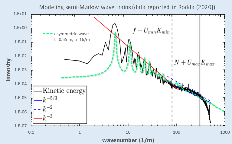
The fit to first-order does show all the harmonics of the fundamental so it is definitely a skewed waveform (as a symmetric waveform would show only the odd harmonics). Yet the peaks are too sharp, and likely the width of the spectral lobes is due to the sampling being limited to a few cycles. By fitting to a cusped asymmetric sawtooth-like waveform of ~4 cycles (shown in the upper right inset in the figure below), the power spectra can be duplicated precisely, as shown in the figure below with the model shown in PURPLE.

The extra side-lobes are due to fixed sampling size, so am sure that this is close to the actual waveform shape. One author of the presentation seems to agree — after adding these observations to the comment page, he said:

“thank you very much for your interesting comments. You are right, due to the length of the measured time series the low-frequency wave part is indeed limited to a few waves and also the skewness of the wave form you have shown seems to be rather realistic to me. The low-frequency part consists of Rossby waves (or their relatives, Eady waves) and the cold front is usually steeper as the warm front of the wave.“

Uwe Harlander, 12 May 2020

The point is that the more you can characterize the data the better that you can extract and discriminate the finer structure that you are interested in — in this case, to extract the high wavenumber turbulence one must first distinguish the highly-ordered wave components.

Moreover, this kind of analysis provides confidence that other atmospheric and oceanic gravity wave features [3] can be similarly characterized — as other EGU presentations [4] focus on a similar lab-based experimental apparatus to understand these type of waves. Consider my comments here, as phenomena such as QBO may be simple enough to understand without resorting to a limited physical emulation.

References

1. Rodda, C. & Harlander, U. Transition from geostrophic flows to inertia-gravity waves in the spectrum of a differentially heated rotating annulus experiment. https://meetingorganizer.copernicus.org/EGU2020/EGU2020-9374.html (2020) doi:10.5194/egusphere-egu2020-9374.
2. Nastrom, G. & Gage, K. S. A climatology of atmospheric wavenumber spectra of wind and temperature observed by commercial aircraft. Journal of the atmospheric sciences42, 950–960 (1985).
3. Bushell, A. C. et al. Parameterized Gravity Wave Momentum Fluxes from Sources Related to Convection and Large-Scale Precipitation Processes in a Global Atmosphere Model. http://dx.doi.org/10.1175/JAS-D-15-0022.1 https://journals.ametsoc.org/doi/abs/10.1175/JAS-D-15-0022.1 (2015) doi:10.1175/JAS-D-15-0022.1.
4. Léard, P., Lecoanet, D. & Le Bars, M. A multi-wave model for the Quasi-Biennial Oscillation: Plumb’s model extended. https://meetingorganizer.copernicus.org/EGU2020/EGU2020-7375.html (2020) doi:10.5194/egusphere-egu2020-7375.