In Chapter 12 of the book, we did not delve into the details of the spatial aspects of the LTE-based ENSO standing wave model to any great degree. We did include a concise derivation of the steps involved in creating separable equations, corresponding to solutions for the temporal and spatial parts of the standing wave dipole. However, only passing mention was made of the unique nature of the spatio-temporal coordination which emerges from the model — and which should be observed in the empirically observed behavior. We can do that now with the abundance of comprehensive data available.
In solving Laplace’s Tidal Equations (LTE) as described in Chapter 11, the separation of the partial differential equation leads to a family of terms (akin to a Fourier series)
sin(a f(t)) sin(C a x) + sin(b f(t)) sin(C b x) + ...
where f(t) is the (possibly complex) tidal forcing and a & b are the two lead terms in any model fit, corresponding to the main dipole waveform and the next higher wavenumber solution.
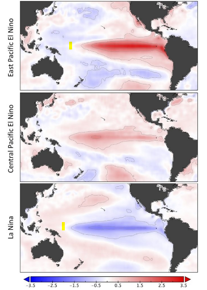
Although the temporal terms are nonlinear and potentially complex, each spatial term is simply a sine wave with a wavenumber proportional to the corresponding a,b,.. values used in the temporal term, with a phase aligned to the oceanic boundary conditions, much as a dynamic electromagnetic field will form a standing wave due to the boundary conditions of the enclosing waveguide or cavity (see e.g. the eastern Pacific boundary condition and dipole node location shown in Figure 1).
The diagrams below are idealized versions of what would happen if the standing wave was driven by a single sine wave without harmonics. Figure 2 is a stacked representation of the oscillating dipole. As this type of figure can get busy very quickly, we opt for an alternate representation. So in Figure 3 is a Hovmoller diagram (time-longitude plot) of the thermocline depth anomalies on the equator, taken from a modeled ocean response to oscillatory winds in a shallow-water model due to Fedorov [1]. In comparison, on the right is an equivalent Hovmoller diagram constructed from a simple LTE model with a single forcing cycle, i.e. f(t)=sin(t) inserted in the first equation above.


The geographical representation of the standing wave dipole is shown in Figure 4 with the SOI measuring points indicated and the dipole node (i.e. zero-crossing point) pointed to by the arrow.
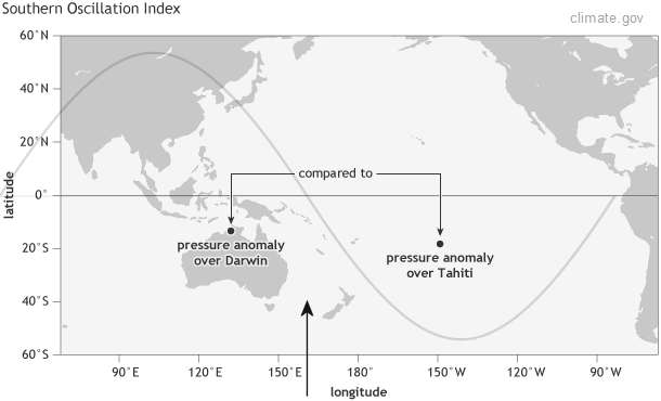
So the a term in the first equation is locked to a dipole that spans the equatorial Pacific, with the node crossing at a longitudinal location in between Darwin and Tahiti denoted by the arrow. All the other higher wavenumber factors scale from the temporal to spatial domain accordingly (via the fixed C term). Each additional wavenumber solution is essentially a spatial harmonic of the main dipole.
Thus, when we do the time-domain fit of ENSO while keeping track of all terms a,b,… , the spatial result is automatically set in place, apart from aligning the phase and selecting the spatial scaling factor C.
Figure 5 below is an initial stab at a spatially aligned fit of the generated standing wave as a Hovmoller diagram, with the left side measurements from [2] (equatorial monthly mean SST anomalies) and the right side computed directly from the LTE-based model fit to NINO34 data collected from 1880-2018.
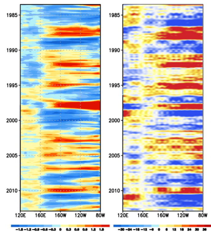
The dipole node is centered around 160E. The faster cycles in the model are likely related to the formation of Tropical Instability Waves, which have some character of a traveling wave. A possible source of the fine structure may also be via ocean currents; as can be seen in Figure 6, the fine detail in the currents appears similar to a cross-section of our LTE model, shown as the horizontal inset pointed to by the arrows.
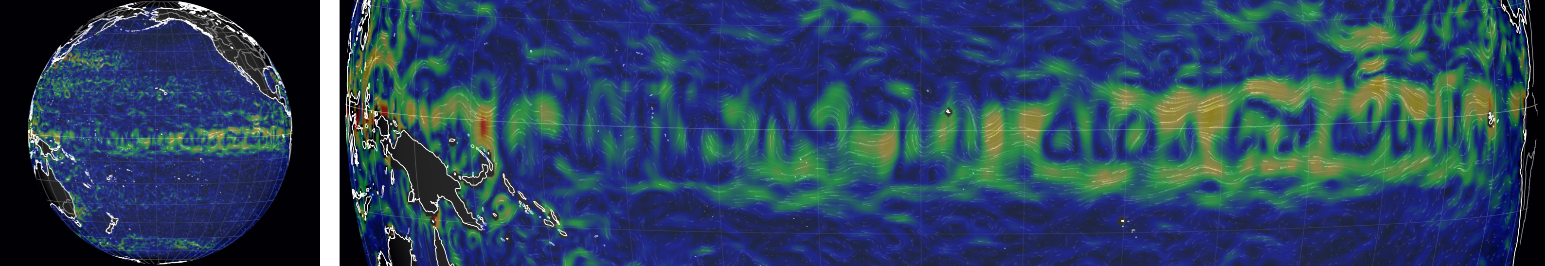
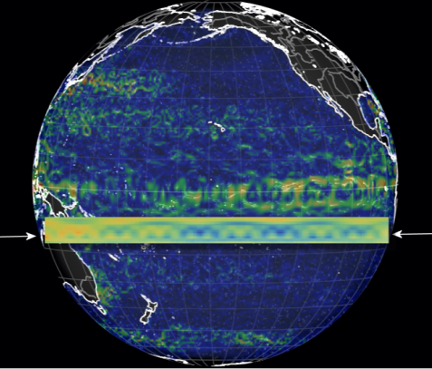
Rectangular inset is a comparison to the LTE model for a time slice.
Some of this data may be available from AVISO. It may take this to reveal the fine structure that may be missing from the observations of Figure 5 if that was averaged over several latitudes about the equator.
References
[1] Fedorov, Alexey V, and Jaclyn N Brown. “Equatorial Waves.” In Ocean Currents, Ed. J. H. Steele, S. A. Thorpe, and K. K. Turekian. Elsevier Science, 2010. http://people.earth.yale.edu/sites/default/files/files/Fedorov/50_Fedorov_EqWaves_Encyclopedia_2009.pdf.
[2] Pinker, R. T., S. A. Grodsky, B. Zhang, A. Busalacchi, and W. Chen. “ENSO Impact on Surface Radiative Fluxes as Observed from Space: ENSO IMPACT ON SURFACE RADIATIVE FLUXES.” Journal of Geophysical Research: Oceans 122, no. 10 (October 2017): 7880–96. https://doi.org/10.1002/2017JC012900.

Very nice interactive site for experimenting with standing or traveling waves
https://www.desmos.com/calculator/i66i9qu1wz
LikeLike
Here is an animation of a surface contour representation of the standing wave ENSO dipole over the 1880-2013 period
LikeLike
Some analysis of Hovmoller diagrams
[1]J. Slawinska, A. Ourmazd, and D. Giannakis, “A New Approach to Signal Processing of Spatiotemporal Data,” in 2018 IEEE Statistical Signal Processing Workshop (SSP), Freiburg im Breisgau, Germany, 2018, pp. 338–342.
https://www.aviso.altimetry.fr/es/data/data-access/las-live-access-server/lively-data/2003/dec-22-2003-longitude-time-diagram-2.html
LikeLike
Hovmoller plot of TIW currents showing the fine structure that the model on the right-side Figure 5 may also revealing.
Traveling waves are along slanted contours while standing waves are horizontal
From Perigaud of NASA JPL:
Click to access perigaud.pdf
LikeLike
SMOS Sea Surface Salinity signals of tropical instability
waves
Xiaobin Yin, Jacqueline Boutin, Gilles Reverdin, Tong Lee, Sabine Arnault,
Nicolas Martin
https://hal.sorbonne-universite.fr/hal-01103198/document
LikeLike
Pingback: Triad Waves | GeoEnergy Math