[mathjax]Here is an alternate derivation of reducing Laplace’s tidal equations along the equator. Recall that the behavior of QBO (and ENSO) is isolated to the equator.
For a fluid sheet of average thickness $$D$$, the vertical tidal elevation $$zeta$$, as well as the horizontal velocity components $$u$$ and $$v$$ (in the latitude $$varphi$$ and longitude $$lambda$$ directions).
This is the set of Laplace’s tidal equations (wikipedia). Along the equator, for $$varphi$$ at zero we can reduce this.
![{begin{aligned}{frac {partial zeta }{partial t}}+{frac {1}{acos(varphi )}}left[{frac {partial }{partial lambda }}(uD)+{frac {partial }{partial varphi }}left(vDcos(varphi )right)right]=0,\{frac {partial u}{partial t}}-vleft(2Omega sin(varphi )right)+{frac {1}{acos(varphi )}}{frac {partial }{partial lambda }}left(gzeta +Uright)=0,\{frac {partial v}{partial t}}+uleft(2Omega sin(varphi )right)+{frac {1}{a}}{frac {partial }{partial varphi }}left(gzeta +Uright)=0,end{aligned}}](https://s0.wp.com/latex.php?latex=%7Bbegin%7Baligned%7D%7Bfrac+%7Bpartial+zeta+%7D%7Bpartial+t%7D%7D%2B%7Bfrac+%7B1%7D%7Bacos%28varphi+%29%7D%7Dleft%5B%7Bfrac+%7Bpartial+%7D%7Bpartial+lambda+%7D%7D%28uD%29%2B%7Bfrac+%7Bpartial+%7D%7Bpartial+varphi+%7D%7Dleft%28vDcos%28varphi+%29right%29right%5D%3D0%2C%5C%7Bfrac+%7Bpartial+u%7D%7Bpartial+t%7D%7D-vleft%282Omega+sin%28varphi+%29right%29%2B%7Bfrac+%7B1%7D%7Bacos%28varphi+%29%7D%7D%7Bfrac+%7Bpartial+%7D%7Bpartial+lambda+%7D%7Dleft%28gzeta+%2BUright%29%3D0%2C%5C%7Bfrac+%7Bpartial+v%7D%7Bpartial+t%7D%7D%2Buleft%282Omega+sin%28varphi+%29right%29%2B%7Bfrac+%7B1%7D%7Ba%7D%7D%7Bfrac+%7Bpartial+%7D%7Bpartial+varphi+%7D%7Dleft%28gzeta+%2BUright%29%3D0%2Cend%7Baligned%7D%7D+&bg=ffffff&fg=444444&s=0&c=20201002)
where $$Omega$$ is the angular frequency of the planet’s rotation, $$g$$ is the planet’s gravitational acceleration at the mean ocean surface, $$a$$ is the planetary radius, and $$U$$ is the external gravitational tidal-forcing potential.
The main candidates for removal due to the small-angle approximation along the equator are the second terms in the second and third equation. The plan is to then substitute the isolated $$u$$ and $$v$$ terms into the first equation, after taking another derivative of that equation with respect to $$t$$.
Taking another derivative of the first equation:
![{begin{aligned}{frac {partial zeta }{partial t}}+{frac {1}{a}}left[{frac {partial }{partial lambda }}(uD)+{frac {partial }{partial varphi }}left(vDright)right]=0,\{frac {partial u}{partial t}}+{frac {1}{a}}{frac {partial }{partial lambda }}left(gzeta +Uright)=0,\{frac {partial v}{partial t}}+{frac {1}{a}}{frac {partial }{partial varphi }}left(gzeta +Uright)=0,end{aligned}}](https://s0.wp.com/latex.php?latex=%7Bbegin%7Baligned%7D%7Bfrac+%7Bpartial+zeta+%7D%7Bpartial+t%7D%7D%2B%7Bfrac+%7B1%7D%7Ba%7D%7Dleft%5B%7Bfrac+%7Bpartial+%7D%7Bpartial+lambda+%7D%7D%28uD%29%2B%7Bfrac+%7Bpartial+%7D%7Bpartial+varphi+%7D%7Dleft%28vDright%29right%5D%3D0%2C%5C%7Bfrac+%7Bpartial+u%7D%7Bpartial+t%7D%7D%2B%7Bfrac+%7B1%7D%7Ba%7D%7D%7Bfrac+%7Bpartial+%7D%7Bpartial+lambda+%7D%7Dleft%28gzeta+%2BUright%29%3D0%2C%5C%7Bfrac+%7Bpartial+v%7D%7Bpartial+t%7D%7D%2B%7Bfrac+%7B1%7D%7Ba%7D%7D%7Bfrac+%7Bpartial+%7D%7Bpartial+varphi+%7D%7Dleft%28gzeta+%2BUright%29%3D0%2Cend%7Baligned%7D%7D+&bg=ffffff&fg=444444&s=0&c=20201002)
Next, on the bracketed pair we invert the order of derivatives (and pull out $$D$$, which may not be right for ENSO where the thermocline depth varies!)
![{begin{aligned}{afrac {partial^2 zeta }{partial t^2}}&+ frac {partial }{partial t} left[{frac {partial }{partial lambda }}(uD)+{frac {partial }{partial varphi }}left(vDright)right]=0,end{aligned}}](https://s0.wp.com/latex.php?latex=%7Bbegin%7Baligned%7D%7Bafrac+%7Bpartial%5E2+zeta+%7D%7Bpartial+t%5E2%7D%7D%26%2B+frac+%7Bpartial+%7D%7Bpartial+t%7D+left%5B%7Bfrac+%7Bpartial+%7D%7Bpartial+lambda+%7D%7D%28uD%29%2B%7Bfrac+%7Bpartial+%7D%7Bpartial+varphi+%7D%7Dleft%28vDright%29right%5D%3D0%2Cend%7Baligned%7D%7D+&bg=ffffff&fg=444444&s=0&c=20201002)
Notice now that the bracketed terms can be replaced by the 2nd and 3rd of Laplace’s equations
![{begin{aligned}{afrac {partial^2 zeta }{partial t^2}}&+ D left[{frac {partial }{partial lambda }}( frac {partial u }{partial t} )+{frac {partial }{partial varphi }}(frac {partial v }{partial t} )right]=0,end{aligned}}](https://s0.wp.com/latex.php?latex=%7Bbegin%7Baligned%7D%7Bafrac+%7Bpartial%5E2+zeta+%7D%7Bpartial+t%5E2%7D%7D%26%2B+D+left%5B%7Bfrac+%7Bpartial+%7D%7Bpartial+lambda+%7D%7D%28+frac+%7Bpartial+u+%7D%7Bpartial+t%7D+%29%2B%7Bfrac+%7Bpartial+%7D%7Bpartial+varphi+%7D%7D%28frac+%7Bpartial+v+%7D%7Bpartial+t%7D+%29right%5D%3D0%2Cend%7Baligned%7D%7D+&bg=ffffff&fg=444444&s=0&c=20201002)

as

![{begin{aligned}{a^2frac {partial^2 zeta }{partial t^2}}&- D left[{frac {partial }{partial lambda }}( {{frac {partial }{partial lambda }}left(gzeta +Uright)} )+{frac {partial }{partial varphi }}({{frac {partial }{partial varphi }}left(gzeta +Uright)})right]=0end{aligned}}](https://s0.wp.com/latex.php?latex=%7Bbegin%7Baligned%7D%7Ba%5E2frac+%7Bpartial%5E2+zeta+%7D%7Bpartial+t%5E2%7D%7D%26-+D+left%5B%7Bfrac+%7Bpartial+%7D%7Bpartial+lambda+%7D%7D%28+%7B%7Bfrac+%7Bpartial+%7D%7Bpartial+lambda+%7D%7Dleft%28gzeta+%2BUright%29%7D+%29%2B%7Bfrac+%7Bpartial+%7D%7Bpartial+varphi+%7D%7D%28%7B%7Bfrac+%7Bpartial+%7D%7Bpartial+varphi+%7D%7Dleft%28gzeta+%2BUright%29%7D%29right%5D%3D0end%7Baligned%7D%7D+&bg=ffffff&fg=444444&s=0&c=20201002)
The $$lambda$$ terms are in longitude so that we can use a separation of variables approach and create a spatial standing wave for QBO, $$SW(s)$$ where $$s$$ is a wavenumber.
![{begin{aligned}{frac {partial^2 zeta }{partial t^2}}&- D left[( SW(s) zeta )+{frac {partial }{partial varphi }}({{frac {partial }{partial varphi }}left(gzeta +Uright)})right]=0end{aligned}}](https://s0.wp.com/latex.php?latex=%7Bbegin%7Baligned%7D%7Bfrac+%7Bpartial%5E2+zeta+%7D%7Bpartial+t%5E2%7D%7D%26-+D+left%5B%28+SW%28s%29+zeta+%29%2B%7Bfrac+%7Bpartial+%7D%7Bpartial+varphi+%7D%7D%28%7B%7Bfrac+%7Bpartial+%7D%7Bpartial+varphi+%7D%7Dleft%28gzeta+%2BUright%29%7D%29right%5D%3D0end%7Baligned%7D%7D+&bg=ffffff&fg=444444&s=0&c=20201002)
The next bit is the connection between a change in latitudinal forcing with a temporal change:

so if

to describe the external gravitational forcing terms, then the solution is the following:

where $$A$$ is an aggregate of the constants of the differential equation.
So we can eventually get to a fit that looks like the actual QBO, for a fit from 1954 to 2015 for the 30 hPa data.

Besides the excursion-limiting behavior imposed by a $$sin(sin(t))$$ modulation, this formulation can also show amplitude folding at the positive and negative extremes. In other words, if the amplitude is too large, the outer $$sin$$ modulation starts to shrink the excursion, instead of just limiting it. Note around the 2016 time frame, the negative peak starts folding inward.
One caveat in this derivation is that the QBO may actually be the $$v(t)$$ term – the horizontal longitudinal velocity of the fluid, the wind in other words – which can be derived from the above by applying the solution to Laplace’s third tidal equation in simplified form above.
EDIT (8/22/2016) — The caveat in the paragraph above is resolved in this post.
What I have derived is a first step, good enough for modeling the QBO for the time being. But the dynamics of ENSO substantially differ in character from the QBO, showing more extreme excursions. How could that come about?
Consider if instead of $$U$$ being a constant, it varies in a similar sinusoidal fashion, then that term will go to the RHS as a forcing, and the above impulse response function will need to be convolved with that forcing . The same goes for the $$D$$ factor which I foreshadowed earlier. Having these vary with time changes the character of the solution. So instead of having a relatively constant amplitude envelope characteristic of QBO, the waveform amplitude will become more erratic, and more similar to the dynamics of ENSO, where the peak excursions vary a considerable amount.
Modifying the $$D$$ factor in fact makes the solution closer to a Mathieu equation formulation. The stratosphere is constant in depth (i.e. stratified) so that’s why we set that to a constant. Yet remember that with ENSO, it is the thermocline depth that is sloshing wildly. The density differences of water above and below the thermocline is what is sensitive to the lunar gravitational forcing. That’s why with a strict biennial modulation applied to the $$D$$ term allows an ENSO model that shows a behavior that matches the data so well:
This is a fit for ENSO from 1880 to 1950, with the validation to the right
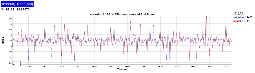
Note how well the amplitudes vary in prediction.
In contrast for QBO, a training run from 1953 to 1983 shows this (this may be sign inverted, I don’t care since the positive direction of QBO is defined arbitrarily):
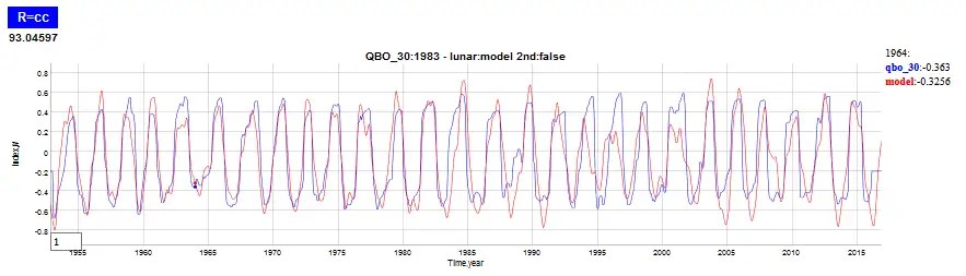
The validated model to the right of 1983 shows much less variation with amplitude, in keeping with the excursion-limiting behavior of the sin-of-a-sin formulation (i.e. $$sin(sin(t))$$).
These kinds of approximations are very common in the physics that I was taught, especially in the hairy world of solid-state physics. Simplifying the starting set of equations will not only reduce complexity but it often brings a level of understanding not normally accessible from looking at the original formulation.

In the sloshing formulation, Frandsen shows how the U(t) gravitational term is modified, U(t)=g+Z”(t), where the vertical acceleration of the moving reference frame adds to the constant gravity term.
This is critical to achieving the Mathieu solution
PDF
LikeLike
And a reminder from Richard Lindzen:
Click to access 18_bet~1.pdf
LikeLike
Ear-ie
LikeLike
Pingback: QBO Model Final Stretch | context/Earth
I don’t even know what to say, this made things so much easier!
LikeLike
If you installed the application from a package file such as *.dmg, then simply go to Application and drag the application to your Trash. You will be prompted to provide your admin password and that’s it. You can then remove any other custom shortcut you may have created on the Dock or other places.
LikeLike
Pingback: Reverse Engineering the Moon’s Orbit from ENSO Behavior | context/Earth
Pingback: Is the SOI noisy or is it signal? | context/Earth
Pingback: Reverse Engineering the Moon’s Orbit from ENSO Behavior | context/Earth
Great blog. Really liked your template. I hope in the future I can have a blog like yours.
LikeLike
Thank you for the sensible critique. Me and my neighbor were just preparing to do a little research about this. We got a grab a book from our local library but I think I learned more clear from this post. I am very glad to see such wonderful information being shared freely out there.
LikeLike
Appreciate it for helping out, wonderful information.
LikeLike
ankara sikis
LikeLike
Hey There. I discovered your blog the usage of msn. That is a very smartly written article. I’ll make sure to bookmark it and come back to learn more of your helpful information. Thanks for the post. I will certainly return.
LikeLike
kurumsal ankara web hosting sizlere en iyi update sunuyor.
LikeLike
Pingback: 000568-000039
Pingback: http://dubailady.hotprovider.com/home
welcomte guzek bir tur
LikeLike