I applied the QBO aliased lunar tidal model to another measure that seems pretty obvious — long term monthly time series data of sea-level height (SLH), in this particular case tidal gauge readings in Sydney harbor (I wrote about correlating Sydney data to ENSO before — post 1 and post 2).
The key here is that I used the second-derivative of the tidal data for the multiple regression fit:
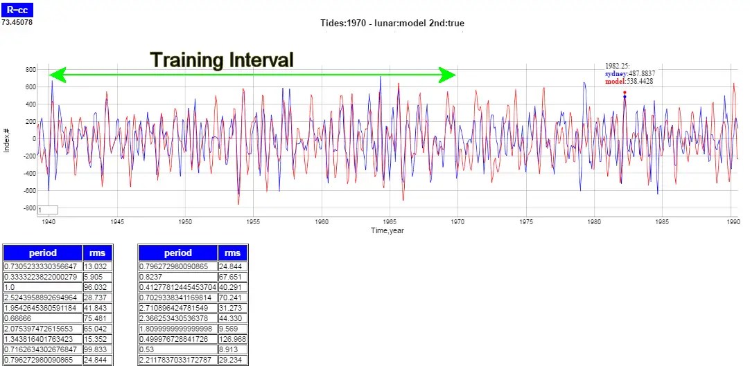
Fig 1: QBO factors over the training interval
This is remarkable as it applies the as-is QBO factors to Sydney training data from 1940 to 1970. That is, the parameters are solely derived from the critical aliased lunisolar periods used to optimize the QBO fit.
The second derivative allows us to fit against a wave equation model.
I don’t know why I didn’t try this earlier, since it’s kind of obvious that whatever lunisolar forces may drive the QBO will certainly drive the sea-level height. Yet I can see why this has been overlooked in the past, since the precise seasonal aliasing of the lunar periods is something that is not intuitively obvious.
Here is another screenshot with an additional low-pass filter applied:
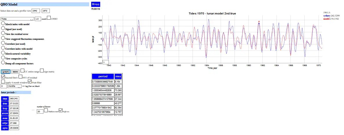
Fig 2: Additional filtering applied to Figure 1
 Remember, this is not the fast diurnal tidal changes as seen to the right, but what is averaged over the course of a month. Clearly some aliasing will occur simply due to the math of artificial aliasing (i.e. a lunar month is shorter than a calendar month), but this still has vast implications for how the data needs to be modeled.
And I think it will help fill in the details for an ENSO model, as the tidal gauge data also shows a hidden correlation to the SOI measure:

Fig 3: This correlation of SLH to SOI uses a 2-year difference applied to the SLH tidal readings to extract the ENSO signal.
What the 2-year differencing does is apply an inexpensive filter to the SLH readings, which is enough to remove most of the quasi-biennial time-series content from the SLH. Thus it reveals the remaining fluctuations in the SLH content, which largely consists of the inverted barometer effect of the standing wave ENSO!
So if we add this ENSO factor to the multiple regression fit of QBO, the correlation will improve even more significantly than shown in Figure 1.
See comments for updates.

The detail in the fit isn’t quite as eye-opening as that for QBO, but with a bit more work, it may yet get there.
There is just so much data available for tides.
LikeLike
Here is the more amazing correlation that the extended SLH readings from Sydney Harbor have with the SOI. This is important because the data for SOI is not uniformly high-quality over the years.
This is the noisy SLH signal that we are dealing with:
What I found was that the yearly and biannual lunisolar signals are cross-modulated by ENSO, and if these form the basis functions for the tidal SLH, then the SLH and SOI time series correlate amazingly well.
Y(t) = yearly and seasonal biannual signal
LOD(t) = long-term angular moment changes (in Length-of-day) that has correlation with temperature
TSI(t) = solar (sunspot) variation
CO2(t) = AGW component
SOI(t) = southern index oscillation
Trying to extract the SOI signal from the SLH signal
(1) SOI(t) = SLH(t) – Y(t) * ( 1 + k*SOI(t) ) – LOD(t) – TSI(t) – CO2(t)
This is admittedly tricky because the cross-terms introduce an automatic correlation. So I’m aware and very sensitive to this issue but its worth the risk to work through it.
Expanded version along the training interval, the two downward dips at 1983 and 1998 are the big El Ninos.
I next grouped the cross-terms on the SOI side (compare to (1) above)
(2) SLH(t) = SOI(t) + Y(t) * ( 1 + k*SOI(t) ) + LOD(t) + TSI(t) + CO2(t)
In the first grouping, look at where the errors in the tidal gauge SLH modulation occur, big spikes at 1905 and 1950 — at the same intervals where I have problems with the ENSO model, see the green shaded region below.
To explain the excursions, either the model is wrong or the data is wrong. It’s possible that the tidal gauge SLH data is telling us that the official SOI readings are erroneous at these points.
LikeLike
Another tidal gauge SLH data set with a long history (1900-2000) is the one from Auckland, NZ. There were a few missing data points so I interpolated over those.
This shows almost identical behavior as the Sydney Harbor set:
After training on the Aukland data, the error excursions at 1905 and 1950 are still there.
LikeLike