[mathjax]In the last post on characterizing ENSO, I discussed the trend I observe in the modeling process — the more I have worked it, the simpler the model has become. This has culminated in what I call a “baby” differential equation model, a model that has been reduced to the bare minimum.

This has partly been inspired by Professor John Carlos Baez’s advice over at the Azimuth Project

“I think it’s important to take the simplest model that does a pretty good fit, and offer extensive evidence that the fit is too good to be due to chance. This means keeping the number of adjustable parameters to a bare minimum, not putting in all the bells and whistles, and doing extensive statistical tests”

Well, I am now working with the bare minimal model. All I incorporate is a QBO forcing that matches the available data from 1953 to current. Then I apply it to a 2nd-order differential equation modeled as a characteristic resonant frequency $$omega_0$$.

$$ f”(t) + omega_0^2 f(t) = Forcing(t) = qbo(t) $$

I adjust the initial conditions and then slide the numerically computed Mathematica output to align with the data.

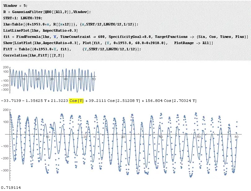
The figure below is the empirical fit to the QBO, configured as a Fourier series so I can extrapolate backwards to 1880.

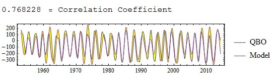
Figure 2 is a fit using the first 400 months of ENSO SOI data as a training interval, and validated to the last 800 months (100 years total)

The next fit uses the second 400 months of data as a training interval, which is then validated forward and backward by 400 months

The final fit using the last 400 months of data, and validates to the first 800 months

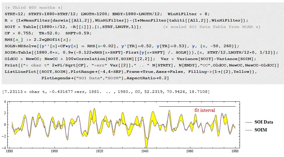
In each case, the overall correlation coefficient is above 0.7, which is as much as can be expected given the correlation coefficient of the empirical model fit to the raw QBO data.

At this point we can show a useful transformation.

$$ f”(t) + omega_0^2 f(t) = qbo(t) $$

If we take the Fourier transform of both sides, then:

$$ (-omega^2 + omega_0^2) F(omega) = QBO(omega) $$

This implies that the power spectra of SOI and QBO should contain many of the same spectral components, but scaled at values proportional to the frequency squared. That is why the SOI, i.e. f(t) or F($$omega$$), contains stronger long time-period components; while the QBO shows the higher frequency, e.g. the principal 2.33 year period, more strongly.

One may ask, what happened to the Chandler wobble component that has been discussed in previous posts?

It is still there but now the wobble forcing is absorbed into the QBO. Using the recently introduced and experimental “FindFormula” machine learning algorithm in Mathematica, the 6+ year Chandler wobble beat period shows up in the top 3 cyclic components of QBO! See the following figure with the yellow highlight. It is not nearly as strong as the 2.33 year period, but because of the spectral scaling discussed in the previous paragraph, it impacts the ENSO time profile as importantly as the higher frequency components.

 Discussion

The caveat in this analysis is that I didn’t include data after 1980, which is explained by the non-stationary disturbance of the climate shift that started being felt after 1980. This will require an additional 400 month analysis interval that I am still working on.

“Can you tell me in words roughly what these 20 lines do, or point me to something you’ve written that explains this latest version?”

It is actually now about half that, if the fitting to the QBO is removed. And the part related to just the DiffEq integration computation is just a couple of lines of Mathematica code. The rest is for handling the data and graphing.

The fit to the QBO can be made as accurate as desired, but I stopped when it got to the correlation coefficient as shown in the first figure above. The idea is that the final modeling result will have a correlation coefficient about that value as well (as the residual is propagating an error signal), which it appears to have.

The geophysics story is very simple to explain, as it is still sloshing but the forcing is now reduced to one observable component. If I want to go this Baby D Model route, I can shorten my current ENSO sloshing paper from its current 3 pages to perhaps a page and a half.

The statistical test proposed is to compare against an alternate model and then see which one wins with an information criteria such as Akaike. I only have a few adjustable parameters (2 initial conditions, a characteristic frequency, and a time shift from QBO to ENSO), so that this will probably beat any other model proposed. It certainly will beat a GCM, which contains hundreds or thousands of parameters