I have previously described a basic thermodynamic model for global average temperature that I call CSALT. It consists of 5 primary factors that account for trend and natural variability. The acronym C S A L T spells out each of these factors.
C obviously stands for excess atmospheric CO2 and the trend is factored as logarithm(CO2).
S refers to the ENSO SOI index which is known to provide a significant fraction of temperature variability, without adding anything by way of a long-term trend. Both the SOI and closely correlated Atmospheric Angular Momentum (AAM) have the property that they revert to a long-term mean value.
A refers to aerosols and specifically the volcanic aerosols that cause sporadic cooling dips in the global temperature measure. Just a handful of volcanic eruptions of VEI scale of 5 and above are able to account for the major cooling noise spikes of the last century.
L refers to the length-of-day (LOD) variability that the earth experiences. Not well known, but this anomaly closely correlates to variability in temperature caused by geophysical processes. Because of conservation of energy, changes in kinetic rotational energy are balanced by changes in thermal energy, via waxing and waning of the long-term frictional processes. This is probably the weakest link in terms of fundamental understanding, with the nascent research findings mainly coming out of NASA JPL (and check this out too).
T refers to variations in Total Solar Irradiance (TSI) due mainly to sunspot fluctuations. This is smaller in comparison to the others and around the level predicted from basic insolation physics.
Taken together, these factors account for a correlation coefficient of well over 90% for a global temperature series such as GISTEMP.
Over time I have experimented with other factors such as tidal periodicities and other oceanic dipoles such as North Atlantic Oscillation, but these are minor in comparison to the main CSALT factors. They also add more degrees of freedom, so they can also lead one astray in terms of spurious correlation. A factor such as AMO contains parts of the temperature record itself so also needs to be treated with care.
My biggest surprise is that more scientists don’t do this kind of modeling. My guess is that it might be too basic and not sophisticated enough in its treatment of atmospheric and climate physics to attract the General Circulation Model (GCM) adherents.
So what follows is a step-by-step decomposition of the NASA GISS temperature record shown below, applying the symbolic regression tool Eureqa as an alternative to the CSALT multiple linear regression algorithm. This series has been filtered and a World War II correction has been applied.

The GISTEMP profile, interval 1940-1944 corrected as a 0.1 adjustment down.
The first step is to add the factors to Eureqa as a set of time series, running from 1880 to 2010. (The AMO only runs to 2010 so was truncated there). Then we instruct Eureqa to include the CSALT factors as algebraically manipulable symbolic terms, in addition to any number of sinusoidal components that it sees fit to include.
GISS = f(CO2, SOI, Aero, LOD, TSI, AAM, AMO)
The strongest component that Eureqa finds in Fig 1 is ln(CO2), immediately raising the correlation coefficient to above 0.93.

Fig 1: ln(CO2) is the strongest component
The next factor along the Pareto complexity curve is LOD, raising the CC to 0.96 (Fig 2).

Fig 2: Adding LOD
At this point, to improve the dynamic range, one can shift CO2 and LOD as known factors and then let Eureqa analyze the resultant residual.
GISS - CO2 - LOD = f(SOI, Aero, TSI, AAM, AMO)
It first suggests an AAM factor, giving a correlation coefficient of 0.61 on the residual (Fig 3).

Fig 3: Residual for AAM
Next the volcanic aerosol factor (Aero) raises the coefficient to 0.67 (Fig 4).

Fig 4: Adding Aerosol factor
The SOI factor helps to register the peaks and valleys strongly as El Ninos and La Ninas modulate the earth’s temperature, raising the CC above 0.7 (Fig 5).

Fig 5: Adding SOI.
Next, the TSI raises the residual CC to 0.73 (Fig 6).

Fig. 6: Adding TSI factor
The remaining fluctuations show modulation aligned with the Atlantic Meridional Oscillation (Fig 7). This was only after the AMO was demodulated of its slowly-varying envelope, applying an 8-year isolation as shown here.

Fig. 7: Adding AMO
The last strong Pareto front contribution is one that Eureqa identified by itself. This is a ~19.5 year period sinusoidal factor that either accentuates the 21-22 year TSI Hale cycle or possibly related to a solar-tidal reinforcing Metonic cycle of 19 years (Fig 8).

Fig. 8: Eureqa also finds a 19.5 year period.
Overall, it is clear that all the detail in the natural fluctuations are explained by a limited set of thermodynamic measures along with the influence of CO2. The introduction of the AMO factor shows how an Atlantic dipole complements the SOI Pacific dipole. Even if this factor, which is based on temperature, was not included, the fit would still be compelling.
Putting the factors together using the values up to 1960 as a training interval, the overall fit is shown in Fig 9.
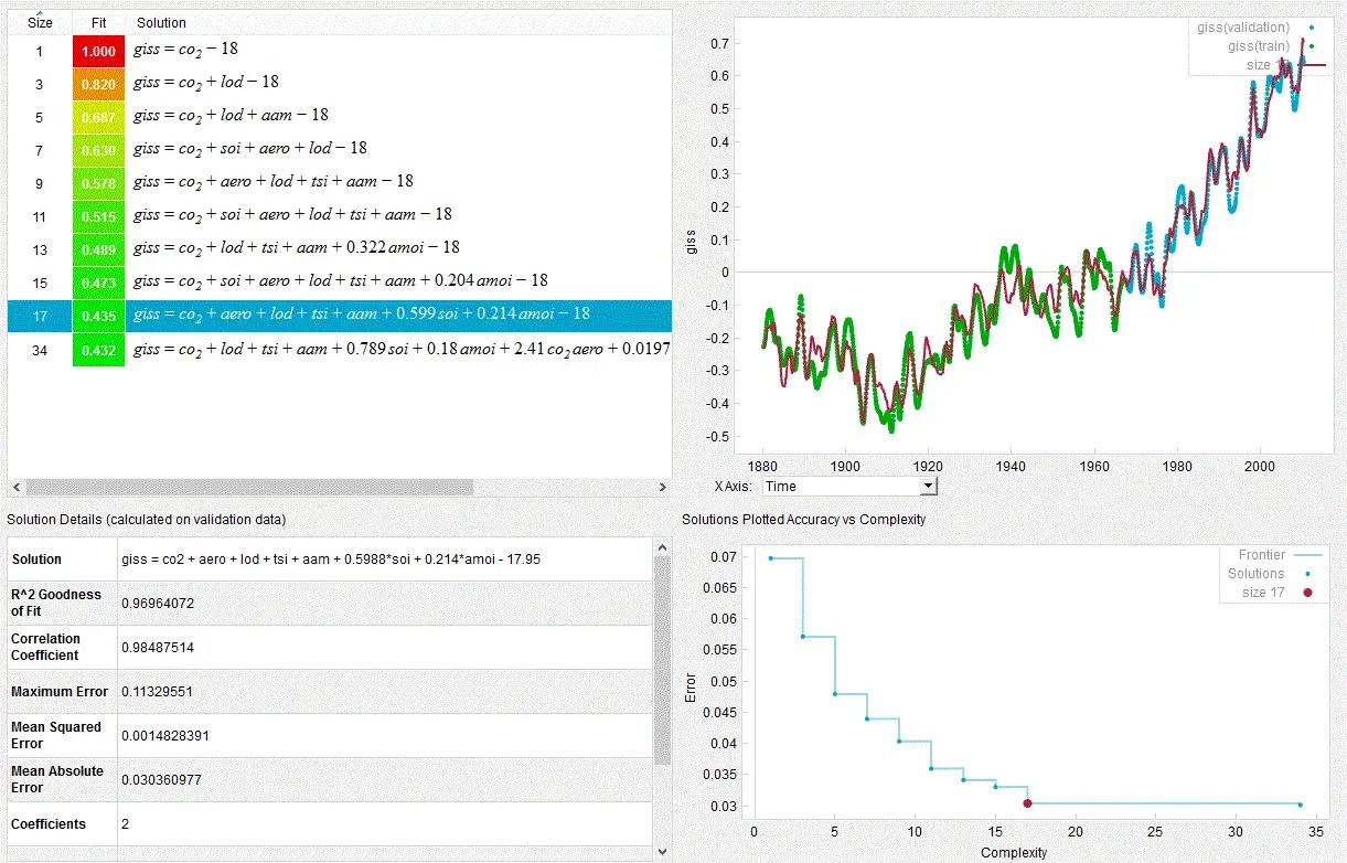
Fig. 9: The traing and validation fit.
Fig 10 is the observed versus predicted regression considering all the factors, showing how well factoring explains both the tend and natural variations. Then with a model such as the SOIM to explain and possibly project fluctuations in the SOI, the approach has potential predictive power as well.

Fig. 10: Observed versus predicted
Eureqa is a very easy tool to use and anyone can apply a CSALT-like of analysis without needing to get bogged sown in the details of mathematical regression techniques.

Did you lag SOI values at all? Because a 6-month lagged SOI correlates with temperatures much better than the unlagged version.
LikeLike
Or actually, 5-month lags work even better, both for HADCRUT and GISS.
LikeLike
Keith, thanks yes I did, the 6 month lag is part of the filter applied to SOI, TSI, and AAM,.
LikeLike
Is the data referenced in these pretty graphs from actual temperature gauge readings or is it the data from after adjustments by the climate change regulators?
I just ask because there has been so much doctoring of temperature data by NOAA/NASA/NCDC and others, that few people trust what they come up with anymore. You should include a disclaimer of why we should trust the data here.
LikeLike
As a libertarian, I am sure you can suggest an organization that will configure the temperature data to your liking, eh?
The word hypocrite comes to mind.
LikeLike
“So there remains a justified general bias toward the simpler of two competing explanations. To understand why, consider that for each accepted explanation of a phenomenon, there is always an infinite number of possible, more complex, and ultimately incorrect, alternatives. This is so because one can always burden failing explanations with ad hoc hypothesis. Ad hoc hypotheses are justifications that prevent theories from being falsified.”
http://en.wikipedia.org/wiki/Occam%27s_razor#Ockham
LikeLike
Correlation with log(CO2) still strong with a few variability components.
LikeLike
Pingback: LOD Revisited for CSALT | context/Earth