[mathjax]As with the discussion about the “pause” in global surface temperatures, much consternation exists about the so-called “missing heat” in the earth’s energy budget.
There are three pieces of the puzzle regarding this issue, which collectively have to fit together for us to be able to make sense about the net energy flow.
- The surface temperature time series, see the CSALT model
- Heat sinking via ocean heat content diffusion, see the OHC model
- The land and ocean surface temperatures have an interaction where they can exchange energy
We have an excellent start on the first two but the last requires a fresh analysis. Understanding the exchange of energy is crucial to not getting twisted up in knots trying to explain any perceived deficit in heat accounting.
Consider Figure 1 below where the energy fluxes are shown at a level of detail appropriate for book-keeping. On the left side, we have an energy balance of incoming flux perturbation (Li) and outgoing flux (Lo) for the land area (we don’t consider the existing balance as we assume that is already in a steady state). On the right side we do the same for the sea or ocean area (Si and So).
The question is how do we proceed if we don’t have direct knowledge of all the parameters. The first guess is that they have to be inferred collectively. The complicating factor is that the sea both absorbs thermal energy (heat) into the bulk shown as the OHC arrow, and that some fraction of the latent and radiative heat emitted by the sea surface transfers over to the land. There is little doubt that this occurs as the Pacific Ocean-originating El Nino events do impact the land, while regular seasonal monsoons work to redistribute enormous amounts as rain originating from the ocean and delivered to the land as moist latent energy. So the question mark in the figure indicates where we need to estimate this split.
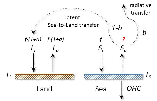
Fig 1: Schematic of energy flow necessary to balance the budget.
Solving this problem would make an excellent homework assignment and perfect for a class in climate science. Let’s give it a try.
Here is a list of parameters that we need to consider
| f | Forcing flux averaged over the earth | ? |
| Li | Incident flux over land | ? |
| Lo | Exit flux from land | ? |
| Si | Incident flux over sea | ? |
| So | Exit flux from sea | ? |
| a | Fraction of incident flux over land above the global average | ? |
| b | Fraction of exiting flux over ocean that radiates to space | ? |
| TL | Average surface temperature anomaly over land | 1.36 (estimated from CSALT model using NOAA data) |
| TS | Average surface temperature anomaly over sea | 0.71 (estimated from CSALT model using NOAA data) |
| PL | Proportion of land area | ? |
| PS | Proportion of sea area | 0.7 |
| OHC | Average net ocean heat content flux | 1 W/m^2 (estimated from OHC model) |
| T | Average global surface temperature anomaly | ? but estimated at 0.90 from CSALT model using NOAA data |
| λ | Climate sensitivity | 0.3 degrees / W/m^2 |
Some of these parameters are measured or estimated but the rest aren’t because of the interactions between the fluxes. To try to solve for their values we need to find or develop equations that map to the problem domain. I count 9 variables so assuming a linear solution, we will need to create 9 or more equations.
| $$ P_L + P_S = 1 $$ | Coverage of land and sea |
| $$ P_L cdot T_L + P_S cdot T_S = T $$ | Mean global surface temperature landsea composite |
| $$ P_L cdot L_i + P_S cdot S_i = f $$ | Globally averaged forcing perturbation |
| $$ L_i = f cdot (1 + a) $$ | Definition of incoming land flux relative to average forcing |
| $$ S_i = f $$ | Definition of incoming sea flux relative to average forcing |
| $$ L_i = L_o $$ | No missing heat on land (limited heat sinking) |
| $$ f cdot a cdot P_L = S_o cdot (1-b) cdot P_S $$ | Transfer from sea to land (* fixed see note at bottom) |
| $$ T_L = lambda cdot L_o $$ | Climate sensitivity definition for land |
| $$ T_S = lambda cdot S_o cdot b$$ | Climate sensitivity definition for sea |
| $$ S_i = OHC + S_o $$ | Conservation of energy flux at the sea surface |
We could solve this with a linear equation solver but the equations appear sparse enough that it is less effort to do the substitutions manually. Take the easy ones first:
$$ P_L = 1 – P_S = 1 – 0.7 = 0.3 $$
and
$$ P_L cdot T_L + P_S cdot T_S = {0.3} cdot {1.36} + 0.7 cdot 0.71 = T = 0.905 $$
which matches the estimate from CSALT. This makes sense because that is also how NOAA does the kriging estimate.
If we continue to make substitutions, we arrive at the expanded form for the transfer equation
$$ (frac{T_L}{lambda} – S_o – OHC) P_L = (S_o – frac{T_S}{lambda}) P_S $$
rearranging terms and using the proportional area identity, we can solve for So
$$ S_o = (frac{T_L}{lambda} – OHC) P_L + frac{T_S}{lambda} P_S $$
and f follows from the last equation
$$ f = S_o + OHC $$
and then a and b derived from the climate sensitivities
$$ a = frac{T_L}{lambda f} – 1 $$
$$ b = frac{T_S}{lambda S_o} $$
Based on the values in the first table, we get a value of 0.22 or 22% for a and a value of 0.87 or 87% for b. The incoming flux is therefore increased from approximately 3.7 W/m^2 to over 4.5 W/m^2 over land as it absorbs moisture from the ocean. By the same token 87% of the non-heat-sunk incoming flux over the ocean is diverted to space, with the remainder of this transferred to land. These values seem reasonable as 13% indicates the level of diversion of latent heat from ocean that we would expect, and 22% is reasonable in terms of amplification of warming that we could intuit.
The value of OHC is estimated in the diffusional model based on the limited data of Levitus [1] and Balmaseda [2]. One can change this number and the energy balance equations would work to correct any deficit of heat. As Trenberth has explained, the OHC numbers are crucial to being able to close the energy budget and also to calibrate the satellite readings such as from the ERBE/CERES experiments (which though precise in relative terms are not that accurate in absolute value).
This analysis resolves a couple of issues. First, it explains why the land surface is warming at twice the rate of the ocean surface — in spite of the smaller than anticipated OHC rate of increase. Secondly, it explains how the “missing heat” is a confusion in how the excess thermal energy gets redistributed by latent actions due to the significant evapotranspiration mechanism at the oceans surface as shown below in Figure 2 (see [3]). It is no coincidence that the evapotranspiration rate of 80 divided by the surface radiation of 396 (calculated as 80/(396+80) = 0.17) shown is consistent with the 13% predicted by the above analysis. That is the amount of latent energy that could be transported to the land. Like I said, all these pieces fit tightly as a jigsaw puzzle.

Fig 2 : Trenberth’s energy budget, showing the net absorbed energy and the significant evapotranspiration at the ocean’s surface.
The rest is uncertainty in the calculation of OHC. Yet in store, I will use the CSALT model to drive the OHC dispersive diffusion formulation (see interactive view) to create a comprehensive view of the earth’s climate. Fun times ahead in climate science, not “seeming a bit boring”, as climatologist Curry has suggested.
References
[2] M. A. Balmaseda, K. E. Trenberth, and E. Källén, “Distinctive climate signals in reanalysis of global ocean heat content,” Geophysical Research Letters, 2013.
[3] It is still possible that negative feedback in the lapse rate can provide further refinement in the analysis, by providing a difference between ocean and land radiative effects, but that would be a second-order correction. Something different between the moisture in the ocean versus moisture over the land would have to occur (possibly due to cloud formation) for this not to be incorporated in the general CO2 control knob theory of climate sensitivity. See the following link for further info: http://www.ipcc.ch/publications_and_data/ar4/wg1/en/ch8s8-6-3-1.html
Added 1/30/2014
(*) In the second table, the equation for sea-to-land energy transfer was mis-transcribed by me as:
$$ f cdot (1+a) cdot P_L = S_o cdot (1-b) cdot P_S $$
Commenter DC used this in his own verification and got the wrong result. I left out the implicit part in the diagram that f*p is coming in as a forcing. Two arrows coming in, one from the ocean and one from the external forcing : (1) f*p and (2) f*a*p, so total incoming = f*p+f*a*p, while going out is f*(1+a)*p. So we only take the f*a*p term and equate that to what is coming from the ocean.
Thanks to DC.

Paul,
Very nice. I am going to have to work through it a few times to make sure I fully understand. Usually I get pretty fuzzy when you start using calculus and differential equations. No excuses here as it is just algebra. I re read the OHC model and that is a pretty heavy lift for my very rusty math skills, but if I start with the assumption that all the math works correctly in that model, getting the model presented here straight should not be a problem. I will no doubt be back later with questions. Thanks.
DC
LikeLike
Thanks DC. This is one of those analyses I was meaning to do for awhile. The original intuition was that since land was heating at twice the rate of the sea, and with the rate of land heating corresponding to 4 W/m^2, the expectation was that 2 W/m^2 was getting sunk into the ocean depths. That would preserve the ratio. But when they measure the ocean sinking only 1 w/m^2, something must be up.
So the idea was to funnel a fraction of the ocean heat onto land and see how the math worked out.
The kicker in this is that we know the SOI plays a role in land heating and so this is one way to get that behavior to jive.
Enough energy gets transferred to land that it can actually change the sea level
http://www.climatecentral.org/news/floods-in-australia-briefly-slowed-sea-level-rise-study-finds-16373
Latest OHC measurements:
http://davidappell.blogspot.com/2014/01/is-ocean-heat-content-accelerating.html
LikeLike
Ok, I think I am fairly clear on the analysis, though I must admit that my calculus skills have become very weak, haven’t really needed to use it much over the last 30 years. So getting from one step to the next in the OHC analysis is a big step for me, for now I will take it on faith that your calculus skills are good enough to have gotten this all correct.
I wonder about the climate sensitivity you are using, typically a doubling of CO2 would result in 3.7 W/m^2 of forcing and about a 3 C delta T at equilibrium which would lead to lambda of 0.8. CSalt leads to 2C TCR, which would give lambda of 0.54. It is not clear where lambda=0.3 comes from unless it is a typo.
DC
LikeLike
DC, Good question on the climate sensitivity. There is one sensitivity that is directly related to the Planck response which goes as :
P ~ T^4
where P is the same units as the f-parameter I am using in watts/m^2 of radiation flux intensity.
Differential calculus says
dP ~ 4 * T^3 dT
which is
dP = 4*(P/T)*dT
by back-substitution
dP/dT = 1/lambda = 4*P/T
This comes out to 4* 240W/m^2 / 290K = 3.31 W/m^2 / C
for nominal earth conditions in steady-state with the sun’s solar insolation.
Flipping that we get a lambda of 0.3 degrees C / W/m^2
The widespread misunderstanding comes about when this number is confused with a CO2 sensitivity. That one is change in temperature related to change in CO2, not to radiation flux.
So if CO2 sensitivity is 1.1 C per doubling of CO2, then it would show a
1.1 C / doubling * (1/0.3) W/m^2 / C = 3.7 W/m^2 / doubling of CO2, which is the CO2 sensitivity that you mentioned.
I know this is very confusing due to the number of flavors of climate sensitivity out there, and the fact that they all seem to be about the same value. The critical thing is to look at the units and understand if they refer any implicit doublings.
LikeLike
Ok got it. Climate sensitivity is often used to refer to a response to doubled CO2 as is TCS or ECS, so I got confused. Often the radiative forcing due to increased CO2 in the atmosphere is given in W/m2, upon reading more carefully this is clearly the back radiation shown towards the right side of Trenberth’s diagram (your figure 2), sorry for the dumb question.
DC
LikeLike
I just re-read the Wikipedia on climate sensitivity and realize why I was confused.
I decided Real Climate would be better and read,
“Climate sensitivity is a measure of the equilibrium global surface air temperature change for a particular forcing. It is usually given as a °C change per W/m2 forcing. A standard experiment to determine this value in a climate model is to look at the doubled CO2 climate, and so equivalently, the climate sensitivity is sometimes given as the warming for doubled CO2 (i.e. from 280 ppm to 560 ppm). The forcing from doubled CO2 is around 4 W/m2 and so a sensitivity of 3°C for a doubling, is equivalent to a sensitivity of 0.75 °C/W/m2. The principal idea is that if you know the sum of the forcings, you can estimate what the eventual temperature change will be.”
http://www.realclimate.org/index.php/archives/2004/11/climate-sensitivity/
So it may be that the sensitivity you are using is what is sometimes termed the “no feedback” climate sensitivity. It seems that a sensitivity of at least 0.5 (which is what pops out from CSALT) would make more sense than 0.3. As far as I understand treating the earth as a blackbody misses quite a bit. Does a lambda of 0.3, reflect all of the components in Trenberth’s diagram?
DC
LikeLike
DC,
I think the key in this analysis is that CO2 does not play into it directly, especially the sensitivity to doubling. The important parameters are the relative warming of land versus sea.
Your concern is warranted on this as it so easy to get wrapped around the axle with values that have an implicit dimensionless doubling parameter. It would almost be a good idea to create another unit called “doubling” which can only be cancelled if the complement is provided.
So we look at this:
“The forcing from doubled CO2 is around 4 W/m2 and so a sensitivity of 3°C for a doubling, is equivalent to a sensitivity of 0.75 °C/W/m2.”
That would be 0.75 °C/W/m2/doubling. So the CSALT results so far have to be referenced to a “doubling” and that it is just for CO2. We have about 1.3C change so far, so this is (1.3/3)*doubling expected so far. But like you say, this is just for the CO2.
So we multiply this out
0.75 °C/W/m2/doubling * (1.3/3)*doubling
and see the “doubling” units cancel out and the current value is about 0.325 °C/W/m2, independent of doubling, which is close to the value of 0.3 C/ W/m^2 we initially assumed.
The other confusing part is that we are already at 4 W/m^2 but that is the control knob value where water vapor is multiplied by the CO2 as positive feedback. So when we get up to 3C, the forcing will be closer to 10 W/m^2.
I could have this wrong as well, but it so vital to the analysis, that I stand to be corrected if it is worked out incorrectly.
LikeLike
Hi Paul,
I am not really trying to correct you, I am trying to learn from you. Possibly in the process of teaching, you learn a little as well.
So my thought process on this is that a doubling of CO2 leads to an increase in radiative forcing of about 3.7 W/m2. The effect on global temperature of an instantaneous doubling of atmospheric CO2 (a step change as it were) should be no different than the insolation suddenly increasing by 3.7 W/m2. The temperature response to such an increase in radiative forcing in the CSALT model is approximately 2 C which would be a lambda of 0.54.
I just re-read a chapter in a textbook I bought 10 years ago called “Global Warming:The Complete Briefing”(Third Edition, 2004) by John Houghton. On Page 25 he goes over the response of the Earth to d doubling of CO2 (which he terms the enhanced greenhouse effect). If nothing else changes except temperature, we would expect a temperature change of 1.2C so lambda would be 0.32 in response to the 3.7 W/m2 increase in forcing. So you are correct to use 0.32 for lambda if you want to ignore fast feedbacks such as increases in water vapor and cloud cover in response to increased temperature. It is not clear to me why you would want to ignore the fast feedbacks and the 0.54 value for lambda seems more appropriate.
If you are able to incorporate slower feedbacks to your model such as ocean heating and ice-albedo feedbacks, I would think you would increase lambda to the ECS level of 0.95 (3.5/3.7).
DC
LikeLike
Hi Paul,
I just reread your previous comment. I think CSALT gives a delta T of about 2 C for doubled CO2.
Your coefficient for C is about 3 and ln(2)= 0.693 so
deltaT=3*0.693=2. Forcing=3.7 W/m^2 and lambda=deltaT/Forcing=2/3.7=0.54.
DC
LikeLike
DC,
On land, I am getting 1.36C for a 4.5 W/m^2 amplified change at a less than half doubling so far. So this will push it up to 3C for a TCR when it finishes doubling on land. Any slow feedbacks will then kick in.
It will be up to near 10 W/m^2 for the effective land forcing at that time This is about 3 times the 3.7 because the CO2 is dragging along other GHGs via the control knob.
I just heard today that Myles Allen gave a presentation at the UK Parliament and he said people should stop using sensitivity
http://judithcurry.com/2014/01/28/uk-parliamentary-hearing-on-the-ipcc/#comment-443830
LikeLike
Hi Paul,
I haven’t read the link to the Allen presentation, though I have read some of his work. On the land vs ocean vs global, it seems to me that we should focus on global temperatures and not consider a “land” or “ocean” sensitivity, it is already confusing enough with “no feedback”, “fast feedback”, “equilibrium”, and “earth system” sensitivities. I am no expert, but it seems the fast feedback (which you are calling TCR, which may not be correct) or ECS or maybe the average (which would be about 0.7) should be used for lambda.
At Real Climate I found the quote below at:
http://www.realclimate.org/index.php/archives/2013/01/on-sensitivity-part-I
“In practice, people often mean different things when they talk about sensitivity. For instance, the sensitivity only including the fast feedbacks (e.g. ignoring land ice and vegetation), or the sensitivity of a particular class of climate model (e.g. the ‘Charney sensitivity’), or the sensitivity of the whole system except the carbon cycle (the Earth System Sensitivity), or the transient sensitivity tied to a specific date or period of time (i.e. the Transient Climate Response (TCR) to 1% increasing CO2 after 70 years). As you might expect, these are all different and care needs to be taken to define terms before comparing things (there is a good discussion of the various definitions and their scope in the Palaeosens paper). – See more at: http://www.realclimate.org/index.php/archives/2013/01/on-sensitivity-part-i/#sthash.IaDrGZXU.dpuf”
If Allen is saying we are tying ourselves in knots trying to untangle this mess, I agree.
Click on attached chart to enlarge.
DC
LikeLike
DC,
I think there is one CO2 sensitivity and that is the sensitivity for land where ECS ~ TCR ~ 3C.
The reason it gets depressed over the ocean is because of the heat sink, so that we have to use a TCR of about 1.5C. Then the combined land+ocean TCR is about 2C.
All this is irrelevant if we shift to analyzing the problem in the way described in this blog post. Now we are talking about fractions of energy moving from ocean to land, and the amount sinking into the ocean. Then all we need is the value of f for a given CO2 value (fast feedback for now) and we can make progress.
LikeLike
Hi Paul,
A couple of thoughts. The first is that some of the “missing” energy may be the 1E20 J/year (or 10,000 PJ/year) of planetary ice loss from the arctic sea and Greenland and Antarctic ice sheets. Though this is not very significant relative to the 7E21 J/Year added to the oceans over the last 30 years (roughly two orders of magnitude less so I can see why it was not considered.)
The second thought is that unless I have misunderstood this analysis the slow feedbacks are still missing. It seems important to add that to the analysis. I am looking at data for CO2 and temperature over the period from 20.5 ky BP to 7.3 ky BP, a span of 13,200 years. CO2 increased from 187 PPM to 260 PPM over this period [delta ln(CO2)=0.3296] and temperature rose from
-2.6C to 0.2 C over this period which leads to
8.5 C/ln(CO2)=2.8C/.3296 ln(CO2)
For a doubling of CO2 from 280 ppm to 560 ppm,
ln(CO2)=0.693 so ECS=8.5*0.693=5.9 C
stabilizing CO2 at 400 PPM leads to 3C ECS and 450 PPM leads to 4C ECS (equilibrium climate sensitivity). What is not clear is how long it will take to reach equilibrium. In the past these changes in CO2 levels occurred over 5,000 to 13,000 years, currently we have raised atmospheric CO2 by a similar log level over 200 years. I would think that we have only seen a portion of the fast feedbacks because the rise has been so rapid, coming out of the most recent glacial period CO2 rose “quickly” over 8000 years and the ECS was about 5C over that period. Then CO2 levels decreased slightly over the next 5000 years (from 265 to 260 ppm)and another 1 C of warming occurred due to slow feedbacks over thousands of years. This rise in temperature with little change in CO2 levels raises the ECS to almost 6C. It is difficult to get this extra 1C into the model, but just a model with CO2 using the slow rise in CO2 over 8000 years (from 18000 YBP to 10000 YBP) gets most of the feedbacks. See Chart (click chart for larger view). P-values for intercept and coefficient are E-110 and E-108 (very close to zero), coefficient for CO2 is 9.5 with std error of 0.2.
DC
LikeLike
DC, At this range of response times, I would imagine it might help to use one of the diffusional response curves. Either the dispersive diffusion response or the hyperbolic response that you have used on the Bakken.
These have the fat-tails that will describe a slow-feedback in terms of the ocean. When to bring this in to the analysis is the question.
The slow feedbacks on land and ice are the albedo and land changes.
LikeLike
I look forward to the confirming physical measurements.
LikeLike
How can the energy flux from ocean to land be directly measured?
We don’t have the equivalent of an ammeter we can put in series.
It all has to be inferred from other measures. That remains the difficulty. We just have to keep on grinding away with respect to self-consistency of all the estimates.
LikeLike
Hi Paul,
Could you check your e-mail? I have a question I would like to ask offline.
DC
LikeLike
please resend, no sign of it.
LikeLike
Hi Paul,
In your post you say,
“Based on the values in the first table, we get a value of 0.22 or 22% for a and a value of 0.87 or 87% for b. The incoming flux is therefore increased from approximately 3.7 W/m^2 to over 4.5 W/m^2 over land as it absorbs moisture from the ocean. By the same token 87% of the non-heat-sunk incoming flux over the ocean is diverted to space, with the remainder of this transferred to land. These values seem reasonable as 13% indicates the level of diversion of latent heat from ocean that we would expect, and 22% is reasonable in terms of amplification of warming that we could intuit.”
It is not clear from the post where the 3.7 W/m^2 for incoming flux comes from. Based on conversations we have had, it seems that this might refer to an increase of radiative forcing due to doubled CO2. At present we are only about half way there on the log scale so I believe this number should be 1.85 W/m^2.
Using the Temperatures given in your post for land and ocean (1.36C and 0.71 C), but changing the climate sensitivity (lambda) to 0.54 and reducing the OHC to 0.7 W/m^2 (based on the last 5 years of the ocean heat chart in your OHC post and and ocean area of 3.61*10^14 m^2) I get:
So=1.465 W/m^2, f=2.165 W/m^2, a= 0.163, and b=0.897, note the good agreement of a= 16% and the estimate of 17% from Trenberth, f is fairly close to the expected value of 1.85 W/m^2, climate sensitivity over land is higher than 0.54 due evapotranspiration and is 0.63. I think 0.3 may be too low for lambda and 1 W/m^2 too high for OHC.
DC
LikeLike
Another mistake by me. It is (1-b) that should agree with Trenberth’s paper and in my case it is 10% which is not in very good agreement with Trenberth’s estimate, based on the data I have ( the chart in the OHC post), I still think the 0.7 W/m^2 is a better estimate than Trenberth’s 0.9 W/m^2.
LikeLike
DC,
As a double check on the 3.7 w/m^2, I do get S_o of 2.7.
It was just a coincidence that it happened to be 3.7, which is the no-feedback forcing in case of doubling of CO2.
I hate when the numbers coincidentally match, which can throw you off.
It is still possible that 1 W/m^2 is too high, and 0.85 W/m^2 might be more reasonable. I don’t know if it can go as low as 0.7 W/m^2 though with the latest numbers that are coming in.
LikeLike
Hi Paul,
I wonder if Si=f works with the equation for f two equations up, it seems if P sub L is non-zero both equations cannot be correct.
Also So should not be 2.7 W/m^2 as f is likely between 1.6 and 1.9 W/m^2 the archer website gives about 1.6 W/m^2 and the standard number (3.7 for doubling) would give 1.85 W/m^2. Lambda of about 0.7 and OHC of 0.85 gives reasonable results, but it seems f(land) is f*(1+a) and f(ocean) is So * b and f should be P(land) * f(land) + P(ocean) *f(ocean), but its not quite coming out correctly. I may be missing something.
LikeLike
Another problem I am having is that it seems “a” must be greater than one and b must be less than one for the model to make physical sense. When f=1.7 and OHC=0.85 we get So=0.85. In that case lambda needs to be more than 0.835 and less than 0.8 to meet the constraints on a and b, so there are limits to what numbers will work for OHC. In order to get “a”>1, lambda has to be less than 0.8, I will use 0.75. Then for b to be less than 1 So must be more than 0.95, which means OHC less than 0.76. I will use OHC=0.75. This gives a=0.05 and
b=0.996. If we use f=1.85 W/m^2 these numbers change, in that case we need lambda less than 0.73, I will use 0.7 and OHC can be higher (0.82 W/m^2). I will choose 0.8 for OHC where “a”= 0.05 and “b”=0.966.
LikeLike
DC,
I think TL and TS temperatures would need to adjust in that case. Remember that this is a set of conservation equations that don’t predict the base temperatures, only provide rules on how the energy must be apportioned.
LikeLike
We know TS and TL, we know f, from CO2 levels, we have a rough idea of OHC (though I think the estimate for fig 2 may be based on a doubled CO2), we should be able to estimate lambda. My main point is if realistic values of f are used (1.6 to 1.85 W/m^2) for current CO2 and temperature, then lambda and OHC are constrained to a narrow possible range by this analysis. If lambda is low say 0.6, it requires a lower OHC for the model to make physical sense at current Temperatures and forcing.
LikeLike
I have played around with the numbers some more and lambda=0.6 and OHC=0.49, gives So=1.36 when f=1.85 using TL=1.36 and TS=0.71 we get a=0.225 and b=0.87.
Also I would change f=PL*Li+PS*So*b so that the f=Si won’t conflict.
Finally the effective global forcing is 1.5 W/m^2, reduced from 1.85 due to some of that incoming flux being stored in the ocean, the difference is not equal to OHC due to the transfer of latent heat to land.
LikeLike
I think there is a difference between your lambda and the lambda that is in the post. The lambda in the post is the Planck climate sensitivity, as described by Hansen in the figure below from his book
http://books.google.com/books?isbn=1408820625
Your lambda is the positive feedback “empirical sensitivity” that has a multiplying effect for a given CO2 forcing. This is talked about by Hansen here:
Click to access 0804.1126.pdf
and he estimates this as 3/4 = 0.75 C/ (W/m^2) of forcing. This generates an f of 1.8 W/m^2 for an OHC of 0.85 W/m^2.
So you are absolutely right that if the OHC is too high then the numbers do not make any sense. If lambda was 0.75 as Hansen has estimated from paleo studies, then the OHC has to be at the most 0.85 W/m^2, otherwise the transfer of heat will be from land to ocean instead of ocean to land.
This is brilliant DC, I think you have it. The OHC has to be somewhere between 0.5 and 0.85.
LikeLike
Cool,
I am really just trying to wrap my brain around some of these concepts, I realize the lamba you were using was based on the Stephan-Boltzman Law, but if I am correct that f is about 1.6 to 1.85 W/m^2 at present (considering CO2 only and ignoring all other all other forcing perturbations) then at present day temperature levels relative to pre-industrial temperatures for land and ocean, a lambda of 0.3 does not give sensible results as far as I can tell.
LikeLike
The quote is perfect, I didn’t read it before my previous response, I think I either saw that before or a summary of the same concept. I should remember this from physics, but as I am sure you can tell, my physics is pretty rusty.
LikeLike
This is another good link that explains some of the discrepancy:
http://www.skepticalscience.com/Kevin-Trenberth-travesty-cant-account-for-the-lack-of-warming.htm
Again, hard to tell if that number is just for the oceans or for the entire surface, but assume it is for the ocean. The trade-off is between having a higher lambda and reducing the ocean-to-land transfer versus a lower lambda and increasing the ocean to land transfer.
Clearly for a lambda of 0.75, the highest the OHC can be is 0.85, and so 0.77 for OHC is within this and has much less ocean-to-land heat transfer than a lambda of 0.3.
LikeLike
Using the data at Appell’s blog, the 0.77 W^m2 matches with the average rate of increase (linear fit on his chart that you referenced in your first comment) in OHC over the oceans only. Chart shows slope of 0.877*10^22 J per year, I converted this to Watts(J/s), by dividing by 3600*24*365.25 seconds and then divided the result by 361*10^12 m^2 of ocean area to get 0.77 W/m^2 for OHC. With lambda=0.75, f=1.75W/m^2, a=0.04, b=0.97 for TL=1.36C and TS=0.71C, when OHC=0.77W/m^2.
Don’t you think that Globally averaged forcing perturbation equation should be changed? I have suggested
f=PL*Lo+PS*So*b so that there is not a conflict with Si=f.
LikeLike
DC,
Looks good, thanks.
I have to think about this one some more. Does it change the equations, or just the interpretation?
One interesting development with your numbers are that we no longer need to drive the heat deeper than 2000 m. Based on the OHC dispersive diffusion model, I was allowing about 20% more of the heat to travel below this layer. We know that some will get down there, but because of a slowdown in diffusion rates below the thermocline and into the abyssal waters, there might not be much effective heat capacity available.
LikeLike
The suggested change is just so the math works, you have two equations for f, if PL>0, both equations cannot be true, so this is a suggested change, based more on math than physics.
I also looked at a doubling of CO2 and the temperatures using your CSALT with both orbital boxes checked, no WW2 correction and no smoothing of data, with lambda of 0.75 and OHC adjusted so that f=3.7 we gat about 2C for global warming and about 3C for land warming for fast feedbacks only, clearly the slower feedbacks would bump this up to about 3C for the globe and probably 4.5 C for land, I am not sure about the timeframe though, I am guessing 1000 years or more if we stopped the CO2 rise at 550 PPM. The slow feedbacks I don’t understand very well, (I am not sure if anyone has more than a guess on those.)
LikeLike
DC,
I can’t figure out to effect the change that you recommended. I get the same numbers that you do so am assuming there is another issue that I am not seeing.
LikeLike
Hi Paul,
It has no effect on the results. It is a simple matter of consistency. If Si=f and
PS*Si+PL*Li=f, now substitute f for Si, PS=0.7, and PL=0.3 and and we get
Li=f which is also f*(1+a), so this would only be true in the special case of a=0.
The equation I suggested allows for 0<a<1, which is what we are looking for.
LikeLike
The second equation for f using PL and PS, is not used to generate any results, which is why it seems it is ok, algebraically I am looking for internal consistency in the set of equations, clearly we are not getting a=0 so only the f=Si equation can remain, the other equation for f needs to be changed, I believe my suggestion makes sense mathematically, and my (limited) understanding of the physics suggests that it makes physical sense as well.
LikeLike
Hi Paul,
You had said that you were getting the same numbers as me. So rather than play around with algebra, let’s use numbers.
You presented 2 equations for f. One is just f=Si, the other is based on Si and Li and the relative land area, which I think should be changed to the outgoing net energy flux, Lo and So*b. One way to think of this in energy balance terms is that f is an incoming flux perturbation to the planet (due to increased CO2 levels relative to preindustrial) and this must be balanced by an outgoing energy flux for the system to be in a quasiequilibrium. We use So*b because a portion of the So is transferred to the land through evapotranspiration
(=(1-b)*So).
It almost seems that a second term called f’ needs to be introduced which could be called the effective global forcing.
This effective forcing would be the equation I have defined and is equal to f’=PL*Lo+PS*So*b=1.207 W/m^2 when
PL=0.3, PS=0.7, TL=1.36, TS=0.71, lambda=0.75, OHC=0.77 W/m^2 which leads to So=0.9757, Si=1.747,
a=0.0388, b=0.97, and Li=1.813. It is also possible to leave the original f in your analysis out and say that Li=Si(1+a) where the Si portion is due to the increased back radiation from increased CO2 and the a*Si portion is due to the latent heat transferred from the warm ocean. TG=f”*lambda=
1.2067*0.75=0.905C, which is about what we expect.
So I would either throw out your original f or introduce a new variable called f’ or maybe f sub e or even f sub g for either effective forcing or global forcing or some such term.
LikeLike
DC,
Sounds reasonable. The value of f was chosen by me to make the problem more easily solvable via a variable transformation approach. Once one knows f, then it can be transformed into any other defined factor.
Rolling up a number as an effective value happens all the time, such as in the effective resistance of an electrical black box. One can use the effective values unless something changes internally. In this case it would be incorporating the dynamics of the OHC buffer.
That is essentially the difference between the equivalent resistance of a box and the impedance of the box, the latter of which includes the long-term time response. In the latter case, we will once again have to look at the innards.
LikeLike
see this
LikeLike
Carbon Brief post
https://www.carbonbrief.org/guest-post-why-does-land-warm-up-faster-than-the-oceans
LikeLike